ARIMA
An introduction to ARIMA forecasting with scalecast.
data: https://www.kaggle.com/datasets/rakannimer/air-passengers
blog post: https://towardsdatascience.com/forecast-with-arima-in-python-more-easily-with-scalecast-35125fc7dc2e
[1]:
import pandas as pd
import numpy as np
from scalecast.Forecaster import Forecaster
from scalecast.auxmodels import auto_arima
import matplotlib.pyplot as plt
import seaborn as sns
import warnings
[2]:
df = pd.read_csv('AirPassengers.csv')
f = Forecaster(
    y=df['#Passengers'],
    current_dates=df['Month'],
    future_dates = 12,
    test_length = .2,
    cis = True,
)
f
[2]:
Forecaster(
    DateStartActuals=1949-01-01T00:00:00.000000000
    DateEndActuals=1960-12-01T00:00:00.000000000
    Freq=MS
    N_actuals=144
    ForecastLength=12
    Xvars=[]
    TestLength=28
    ValidationMetric=rmse
    ForecastsEvaluated=[]
    CILevel=0.95
    CurrentEstimator=mlr
    GridsFile=Grids
)
Naive Simple Approach
this is not meant to be a demonstration of a model that is expected to be accurate
it is meant to show the mechanics of using scalecast
[3]:
f.set_estimator('arima')
f.manual_forecast(call_me='arima1')
[4]:
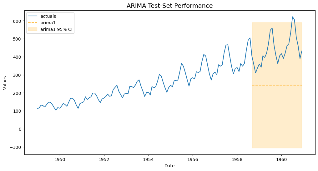
f.plot_test_set(ci=True)
plt.title('ARIMA Test-Set Performance',size=14)
plt.show()
[5]:
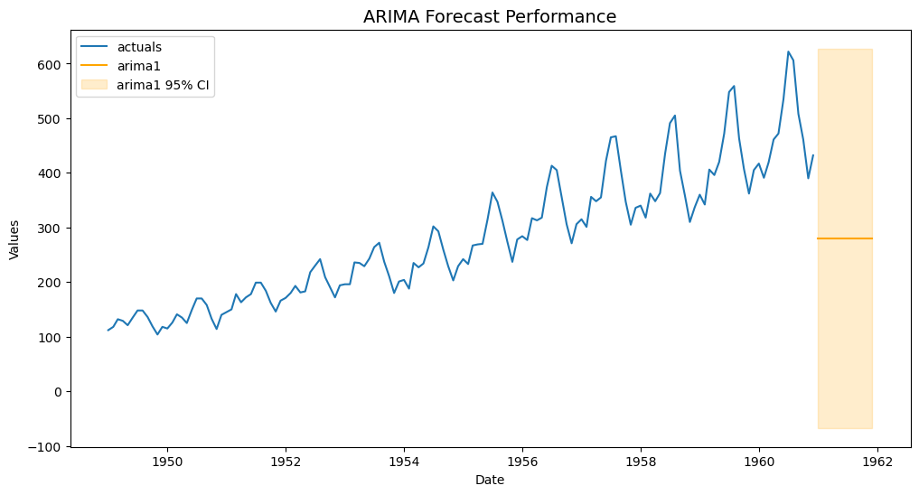
f.plot(ci=True)
plt.title('ARIMA Forecast Performance',size=14)
plt.show()
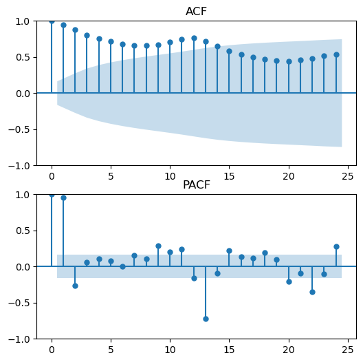
Human Interpretation Iterative Approach
this is a non-automated approach to ARIMA forecasting where model specification depends on human-interpretation of statistical results and charts
[6]:
figs, axs = plt.subplots(2, 1,figsize=(6,6))
f.plot_acf(ax=axs[0],title='ACF',lags=24)
f.plot_pacf(ax=axs[1],title='PACF',lags=24)
plt.show()
/Users/uger7/opt/anaconda3/envs/scalecast-env/lib/python3.8/site-packages/statsmodels/graphics/tsaplots.py:348: FutureWarning: The default method 'yw' can produce PACF values outside of the [-1,1] interval. After 0.13, the default will change tounadjusted Yule-Walker ('ywm'). You can use this method now by setting method='ywm'.
  warnings.warn(
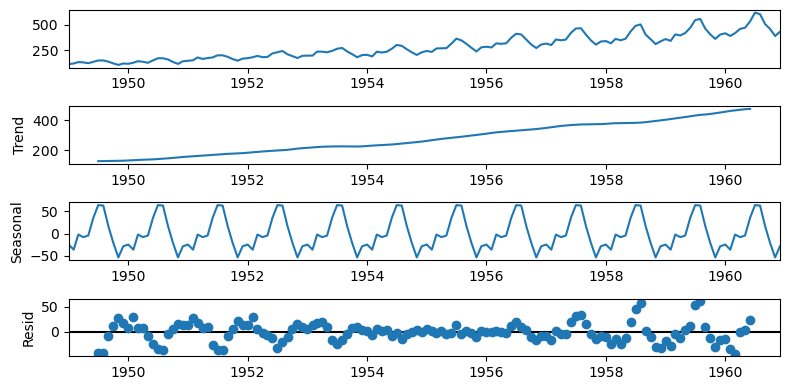
[7]:
plt.rc("figure",figsize=(8,4))
f.seasonal_decompose().plot()
plt.show()
[8]:
stat, pval, _, _, _, _ = f.adf_test(full_res=True)
print(stat)
print(pval)
0.8153688792060442
0.9918802434376409
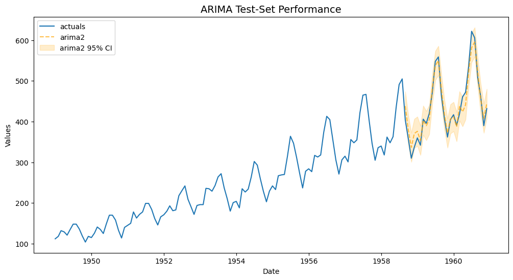
[9]:
f.manual_forecast(order=(1,1,1),seasonal_order=(2,1,1,12),call_me='arima2')
[10]:
f.plot_test_set(ci=True,models='arima2')
plt.title('ARIMA Test-Set Performance',size=14)
plt.show()
[11]:
f.plot(ci=True,models='arima2')
plt.title('ARIMA Forecast Performance',size=14)
plt.show()

[12]:
f.regr.summary()
[12]:
| Dep. Variable: | y | No. Observations: | 144 |
|---|---|---|---|
| Model: | ARIMA(1, 1, 1)x(2, 1, 1, 12) | Log Likelihood | -501.929 |
| Date: | Mon, 10 Apr 2023 | AIC | 1015.858 |
| Time: | 18:47:23 | BIC | 1033.109 |
| Sample: | 0 | HQIC | 1022.868 |
| - 144 | |||
| Covariance Type: | opg |
| coef | std err | z | P>|z| | [0.025 | 0.975] | |
|---|---|---|---|---|---|---|
| ar.L1 | -0.0731 | 0.273 | -0.268 | 0.789 | -0.608 | 0.462 |
| ma.L1 | -0.3572 | 0.249 | -1.436 | 0.151 | -0.845 | 0.130 |
| ar.S.L12 | 0.6673 | 0.160 | 4.182 | 0.000 | 0.355 | 0.980 |
| ar.S.L24 | 0.3308 | 0.099 | 3.341 | 0.001 | 0.137 | 0.525 |
| ma.S.L12 | -0.9711 | 1.086 | -0.895 | 0.371 | -3.099 | 1.157 |
| sigma2 | 111.1028 | 98.277 | 1.131 | 0.258 | -81.517 | 303.722 |
| Ljung-Box (L1) (Q): | 0.00 | Jarque-Bera (JB): | 7.72 |
|---|---|---|---|
| Prob(Q): | 0.99 | Prob(JB): | 0.02 |
| Heteroskedasticity (H): | 2.77 | Skew: | 0.08 |
| Prob(H) (two-sided): | 0.00 | Kurtosis: | 4.18 |
Warnings:
[1] Covariance matrix calculated using the outer product of gradients (complex-step).
Auto-ARIMA Approach
pip install pmdarima
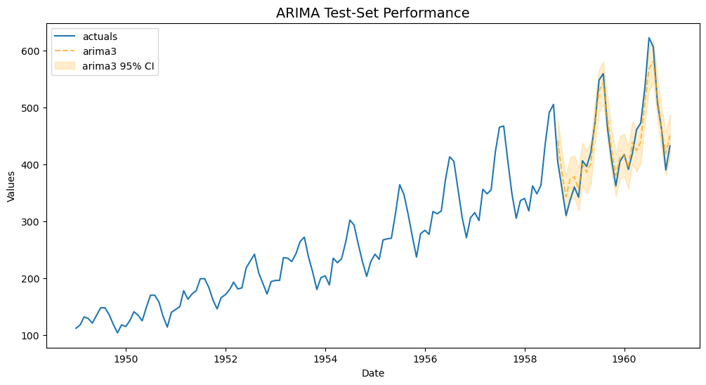
[13]:
auto_arima(
    f,
    m=12,
    call_me='arima3',
)
[14]:
f.plot_test_set(ci=True,models='arima3')
plt.title('ARIMA Test-Set Performance',size=14)
plt.show()
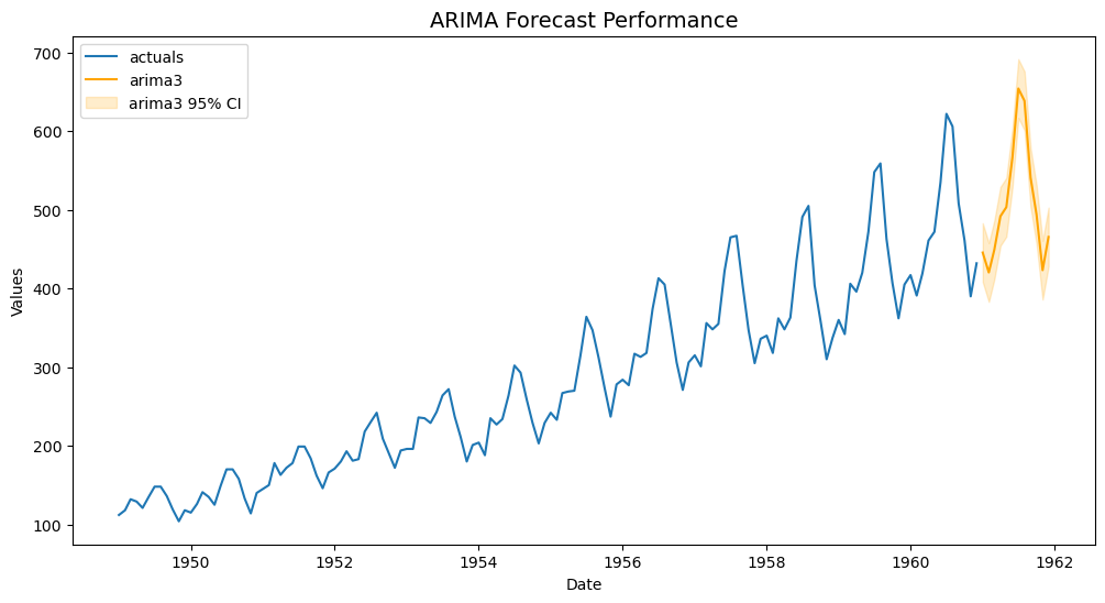
[15]:
f.plot(ci=True,models='arima3')
plt.title('ARIMA Forecast Performance',size=14)
plt.show()
[16]:
f.regr.summary()
[16]:
| Dep. Variable: | y | No. Observations: | 144 |
|---|---|---|---|
| Model: | ARIMA(2, 1, 1)x(0, 1, [], 12) | Log Likelihood | -504.923 |
| Date: | Mon, 10 Apr 2023 | AIC | 1017.847 |
| Time: | 18:47:55 | BIC | 1029.348 |
| Sample: | 0 | HQIC | 1022.520 |
| - 144 | |||
| Covariance Type: | opg |
| coef | std err | z | P>|z| | [0.025 | 0.975] | |
|---|---|---|---|---|---|---|
| ar.L1 | 0.5960 | 0.085 | 6.986 | 0.000 | 0.429 | 0.763 |
| ar.L2 | 0.2143 | 0.091 | 2.343 | 0.019 | 0.035 | 0.394 |
| ma.L1 | -0.9819 | 0.038 | -25.599 | 0.000 | -1.057 | -0.907 |
| sigma2 | 129.3177 | 14.557 | 8.883 | 0.000 | 100.786 | 157.850 |
| Ljung-Box (L1) (Q): | 0.00 | Jarque-Bera (JB): | 7.68 |
|---|---|---|---|
| Prob(Q): | 0.98 | Prob(JB): | 0.02 |
| Heteroskedasticity (H): | 2.33 | Skew: | -0.01 |
| Prob(H) (two-sided): | 0.01 | Kurtosis: | 4.19 |
Warnings:
[1] Covariance matrix calculated using the outer product of gradients (complex-step).
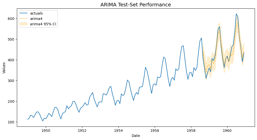
Grid Search Approach
[17]:
f.set_validation_length(12)
grid = {
    'order':[
        (1,1,1),
        (1,1,0),
        (0,1,1),
    ],
    'seasonal_order':[
        (2,1,1,12),
        (1,1,1,12),
        (2,1,0,12),
        (0,1,0,12),
    ],
}

f.ingest_grid(grid)
f.tune()
f.auto_forecast(call_me='arima4')
[18]:
f.plot_test_set(ci=True,models='arima4')
plt.title('ARIMA Test-Set Performance',size=14)
plt.show()
[19]:
f.plot(ci=True,models='arima4')
plt.title('ARIMA Forecast Performance',size=14)
plt.show()

[20]:
f.regr.summary()
[20]:
| Dep. Variable: | y | No. Observations: | 144 |
|---|---|---|---|
| Model: | ARIMA(0, 1, 1)x(0, 1, [], 12) | Log Likelihood | -508.319 |
| Date: | Mon, 10 Apr 2023 | AIC | 1020.639 |
| Time: | 18:50:43 | BIC | 1026.389 |
| Sample: | 0 | HQIC | 1022.975 |
| - 144 | |||
| Covariance Type: | opg |
| coef | std err | z | P>|z| | [0.025 | 0.975] | |
|---|---|---|---|---|---|---|
| ma.L1 | -0.3184 | 0.063 | -5.038 | 0.000 | -0.442 | -0.195 |
| sigma2 | 137.2653 | 15.024 | 9.136 | 0.000 | 107.818 | 166.713 |
| Ljung-Box (L1) (Q): | 0.00 | Jarque-Bera (JB): | 5.46 |
|---|---|---|---|
| Prob(Q): | 0.95 | Prob(JB): | 0.07 |
| Heteroskedasticity (H): | 2.37 | Skew: | 0.02 |
| Prob(H) (two-sided): | 0.01 | Kurtosis: | 4.00 |
Warnings:
[1] Covariance matrix calculated using the outer product of gradients (complex-step).
Export Results
[21]:
pd.options.display.max_colwidth = 100
results = f.export(to_excel=True,excel_name='arima_results.xlsx',determine_best_by='TestSetMAPE')
summaries = results['model_summaries']
summaries[['ModelNickname','HyperParams','InSampleMAPE','TestSetMAPE']]
[21]:
| ModelNickname | HyperParams | InSampleMAPE | TestSetMAPE | |
|---|---|---|---|---|
| 0 | arima2 | {'order': (1, 1, 1), 'seasonal_order': (2, 1, 1, 12)} | 0.044448 | 0.037170 |
| 1 | arima4 | {'order': (0, 1, 1), 'seasonal_order': (0, 1, 0, 12)} | 0.046529 | 0.044054 |
| 2 | arima3 | {'order': (2, 1, 1), 'seasonal_order': (0, 1, 0, 12), 'trend': None} | 0.045081 | 0.045936 |
| 3 | arima1 | {} | 0.442457 | 0.430066 |
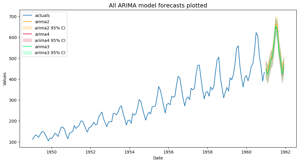
[22]:
f.plot(ci=True,models=['arima2','arima3','arima4'],order_by='TestSetMAPE')
plt.title('All ARIMA model forecasts plotted',size=14)
plt.show()
[ ]: