Introductory Example

This demonstrates an example using scalecast 0.18.0. Several features explored are not available in earlier versions, so if anything is not working, try upgrading:

pip install --upgrade scalecast

If things are still not working, you spot a typo, or you have some other suggestion to improve functionality or document readability, open an issue or email mikekeith52@gmail.com.

Link to dataset used in this example: https://www.kaggle.com/datasets/neuromusic/avocado-prices.

Latest official documentation.

[1]:

import pandas as pd
import numpy as np
import matplotlib.pyplot as plt

[2]:

# read in data
data = pd.read_csv('avocado.csv',parse_dates = ['Date'])
data = data.sort_values(['region','type','Date'])

Univariate Forecasting
Multivariate Forecasting
Transformations
Pipelines
Fully Automated Pipelines
Scaled Automated Forecasting
Exporting Results

Univariate Forecasting

Load the `Forecaster` Object

This is an object that can store data, run forecasts, store results, and plot. It’s a UI, procedure, and set of models all-in-one.
Forecasts in scalecast are run with a dynamic recursive approach by default, as opposed to a direct or other approach.
Forecaster Object Documentation.

[3]:

from scalecast.Forecaster import Forecaster

[4]:

volume = data.groupby('Date')['Total Volume'].sum()

[5]:

f = Forecaster(
    y = volume,
    current_dates = volume.index,
    future_dates = 13,
)

f

[5]:

Forecaster(
    DateStartActuals=2015-01-04T00:00:00.000000000
    DateEndActuals=2018-03-25T00:00:00.000000000
    Freq=W-SUN
    N_actuals=169
    ForecastLength=13
    Xvars=[]
    TestLength=0
    ValidationMetric=rmse
    ForecastsEvaluated=[]
    CILevel=None
    CurrentEstimator=mlr
    GridsFile=Grids
)

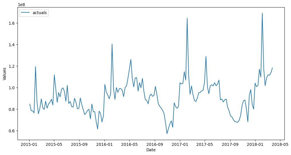
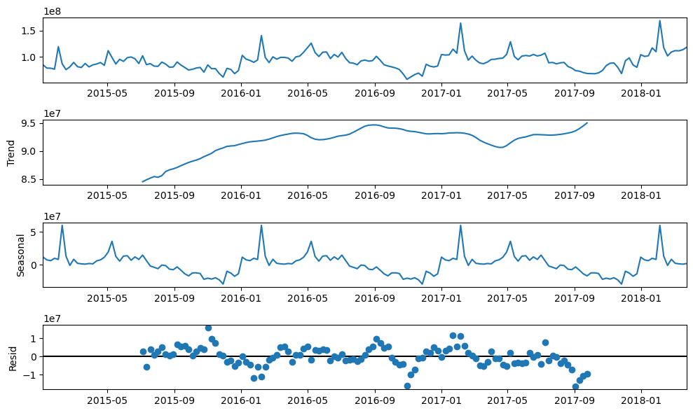
Exploratory Data Analysis

[6]:

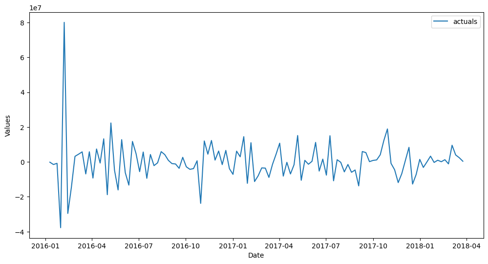
f.plot()
plt.show()

../../_images/misc_introduction_Introduction2_9_0.png

[7]:

plt.rc("figure",figsize=(10,6))
f.seasonal_decompose().plot()
plt.show()

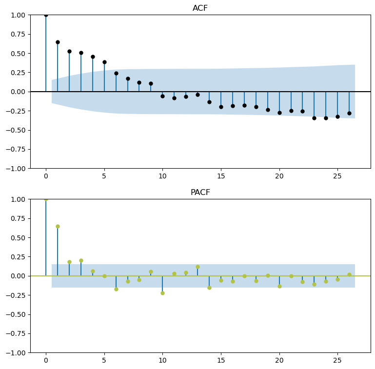
../../_images/misc_introduction_Introduction2_10_0.png

[8]:

figs, axs = plt.subplots(2, 1,figsize=(9,9))
f.plot_acf(ax=axs[0],title='ACF',lags=26,color='black')
f.plot_pacf(ax=axs[1],title='PACF',lags=26,color='#B2C248',method='ywm')
plt.show()

../../_images/misc_introduction_Introduction2_11_0.png

Parameterize the `Forecaster` Object

Set Test Length

Starting in scalecast version 0.16.0, you can skip model testing by setting a test length of 0.
In this example, all models will be tested on the last 15% of the observed values in the dataset.

[9]:

f.set_test_length(.15)

Tell the Object to Evaluate Confidence Intervals

This only works if there is a test set specified and it is of a sufficient size.
See the documentation.
See the example.

[10]:

# default args below
f.eval_cis(
    mode = True, # tell the object to evaluate intervals
    cilevel = .95, # 95% confidence level
)

Specify Model Inputs

Trend

[11]:

f.add_time_trend()

Seasonality

[12]:

f.add_seasonal_regressors('week',raw=False,sincos=True)

Autoregressive Terms / Series Lags

[13]:

f.add_ar_terms(13)

[14]:

[14]:

Forecaster(
    DateStartActuals=2015-01-04T00:00:00.000000000
    DateEndActuals=2018-03-25T00:00:00.000000000
    Freq=W-SUN
    N_actuals=169
    ForecastLength=13
    Xvars=['t', 'weeksin', 'weekcos', 'AR1', 'AR2', 'AR3', 'AR4', 'AR5', 'AR6', 'AR7', 'AR8', 'AR9', 'AR10', 'AR11', 'AR12', 'AR13']
    TestLength=25
    ValidationMetric=rmse
    ForecastsEvaluated=[]
    CILevel=0.95
    CurrentEstimator=mlr
    GridsFile=Grids
)

Run Models

See the available models.
See the blog post.
The dynamic_testing argument for all of these will be 13 – test-set results will then be in terms of rolling averages of 13-step forecasts, which is also our forecast length.
The resulting forecasts from this process are not well-fit. Better forecasts are obtained once more optimization is performed in later sections.

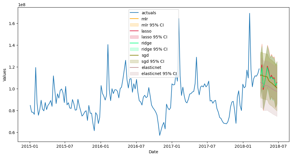
Linear Scikit-Learn Models

[15]:

f.set_estimator('mlr')
f.manual_forecast(dynamic_testing=13)

[16]:

f.set_estimator('lasso')
f.manual_forecast(alpha=0.2,dynamic_testing=13)

[17]:

f.set_estimator('ridge')
f.manual_forecast(alpha=0.2,dynamic_testing=13)

[18]:

f.set_estimator('elasticnet')
f.manual_forecast(alpha=0.2,l1_ratio=0.5,dynamic_testing=13)

[19]:

f.set_estimator('sgd')
f.manual_forecast(alpha=0.2,l1_ratio=0.5,dynamic_testing=13)

[20]:

f.plot_test_set(ci=True,models=['mlr','lasso','ridge','elasticnet','sgd'],order_by='TestSetRMSE')
plt.show()

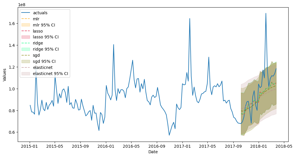
../../_images/misc_introduction_Introduction2_32_0.png

[21]:

f.plot(ci=True,models=['mlr','lasso','ridge','elasticnet','sgd'],order_by='TestSetRMSE')
plt.show()

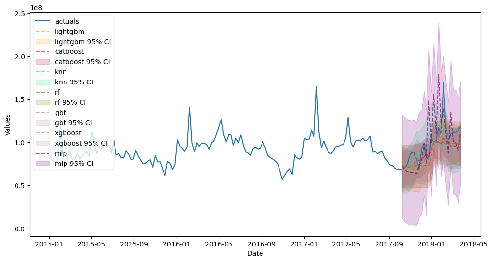
../../_images/misc_introduction_Introduction2_33_0.png

Non-linear Scikit-Learn Models

[22]:

f.set_estimator('rf')
f.manual_forecast(max_depth=2,dynamic_testing=13)

[23]:

f.set_estimator('gbt')
f.manual_forecast(max_depth=2,dynamic_testing=13)

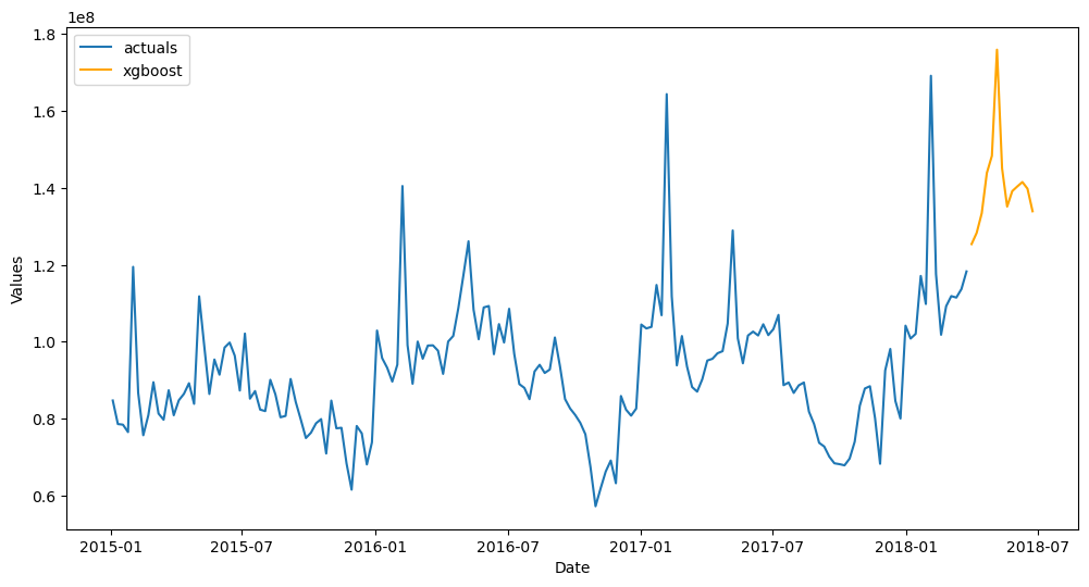
[24]:

f.set_estimator('xgboost')
f.manual_forecast(gamma=1,dynamic_testing=13)

[25]:

f.set_estimator('lightgbm')
f.manual_forecast(max_depth=2,dynamic_testing=13)

[26]:

f.set_estimator('catboost')
f.manual_forecast(depth=4,verbose=False,dynamic_testing=13)

Finished loading model, total used 100 iterations

[27]:

f.set_estimator('knn')
f.manual_forecast(n_neighbors=5,dynamic_testing=13)

Finished loading model, total used 100 iterations

[28]:

f.set_estimator('mlp')
f.manual_forecast(hidden_layer_sizes=(50,50),solver='lbfgs',dynamic_testing=13)

Finished loading model, total used 100 iterations

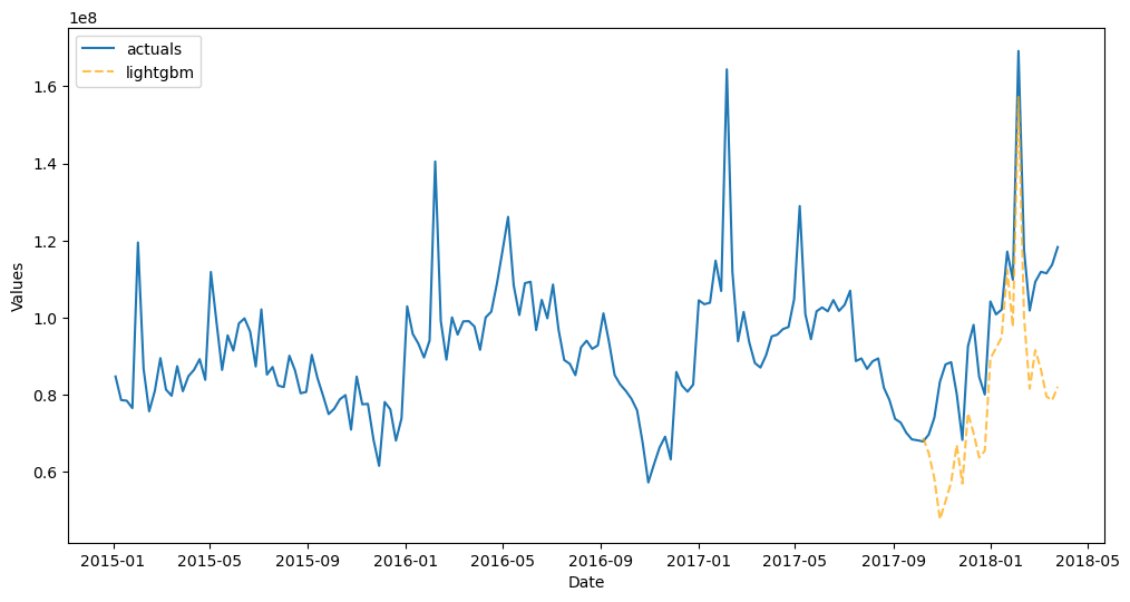
[29]:

f.plot_test_set(
    ci=True,
    models=['rf','gbt','xgboost','lightgbm','catboost','knn','mlp'],
    order_by='TestSetRMSE'
)
plt.show()

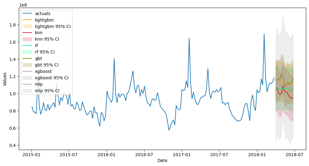
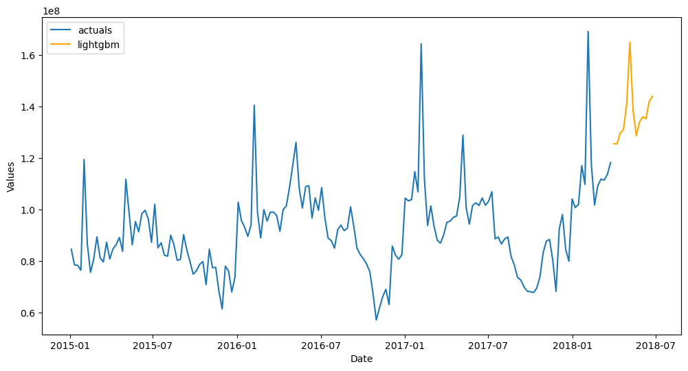
../../_images/misc_introduction_Introduction2_42_0.png

[30]:

f.plot(ci=True,models=['rf','gbt','xgboost','lightgbm','knn','mlp'],order_by='TestSetRMSE')
plt.show()

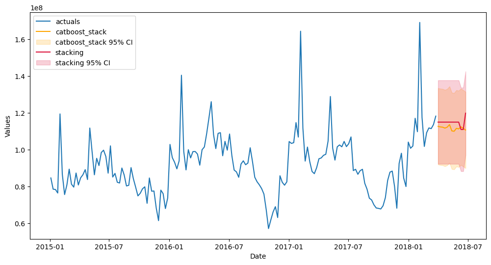
../../_images/misc_introduction_Introduction2_43_0.png

Stacking Models

Sklearn Stacking Model

[31]:

from sklearn.ensemble import StackingRegressor
from sklearn.linear_model import SGDRegressor
from sklearn.linear_model import ElasticNet
from sklearn.ensemble import GradientBoostingRegressor
from sklearn.neighbors import KNeighborsRegressor
from xgboost import XGBRegressor
from lightgbm import LGBMRegressor

[32]:

f.add_sklearn_estimator(StackingRegressor,'stacking')

[33]:

estimators = [
    ('elasticnet',ElasticNet(alpha=0.2)),
    ('xgboost',XGBRegressor(gamma=1)),
    ('gbt',GradientBoostingRegressor(max_depth=2)),
]

final_estimator = LGBMRegressor()

f.set_estimator('stacking')
f.manual_forecast(
    estimators=estimators,
    final_estimator=final_estimator,
    dynamic_testing=13
)

Finished loading model, total used 100 iterations

Scalecast Stacking Model

[34]:

f.add_signals(['elasticnet','lightgbm','xgboost','knn'],train_only=True)
f.set_estimator('catboost')
f.manual_forecast(call_me = 'catboost_stack',verbose=False)

Finished loading model, total used 100 iterations
Finished loading model, total used 100 iterations

[35]:

f.plot_test_set(models=['stacking','catboost_stack'],ci=True,order_by='TestSetRMSE')
plt.show()

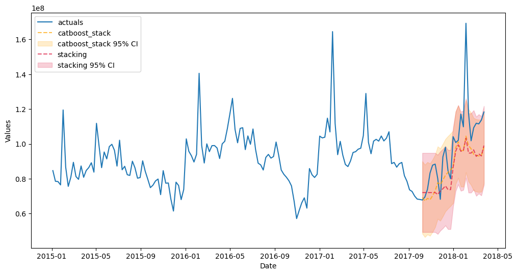
../../_images/misc_introduction_Introduction2_51_0.png

[36]:

f.plot(models=['stacking','catboost_stack'],ci=True,order_by='TestSetRMSE')
plt.show()

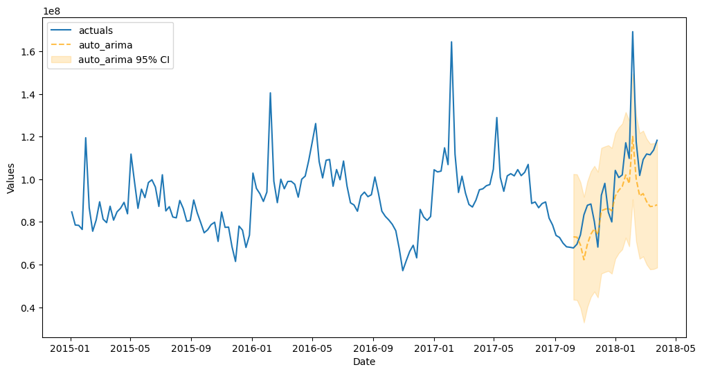
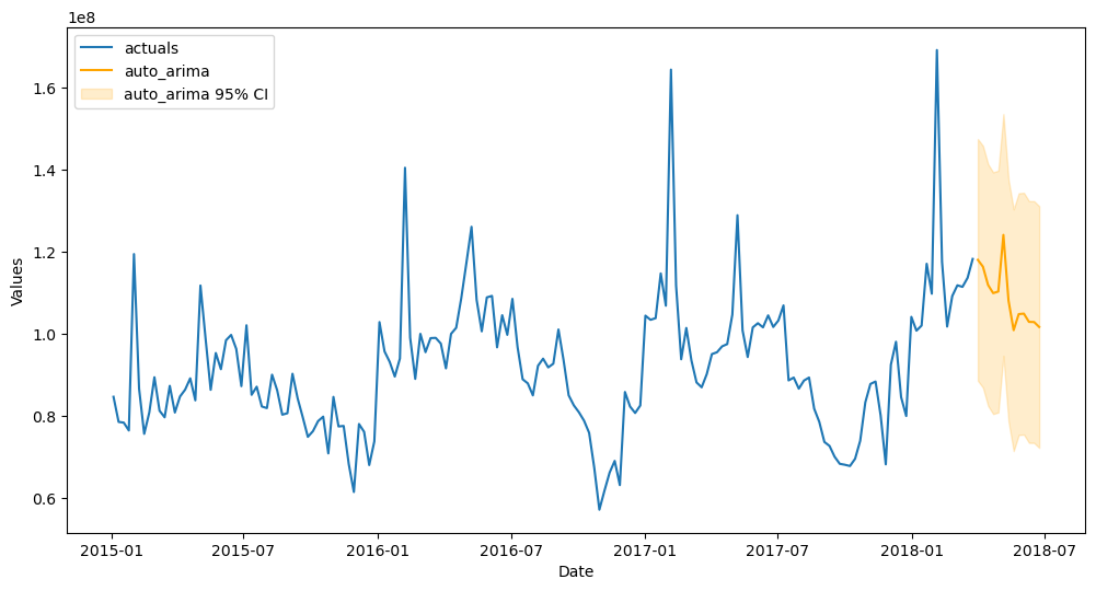
../../_images/misc_introduction_Introduction2_52_0.png

ARIMA

auxmodels.auto_arima

[37]:

from scalecast.auxmodels import auto_arima

[38]:

auto_arima(f,m=52)

Finished loading model, total used 100 iterations
Finished loading model, total used 100 iterations

[39]:

f.plot_test_set(models='auto_arima',ci=True)
plt.show()

../../_images/misc_introduction_Introduction2_56_0.png

[40]:

f.plot(models='auto_arima',ci=True)
plt.show()

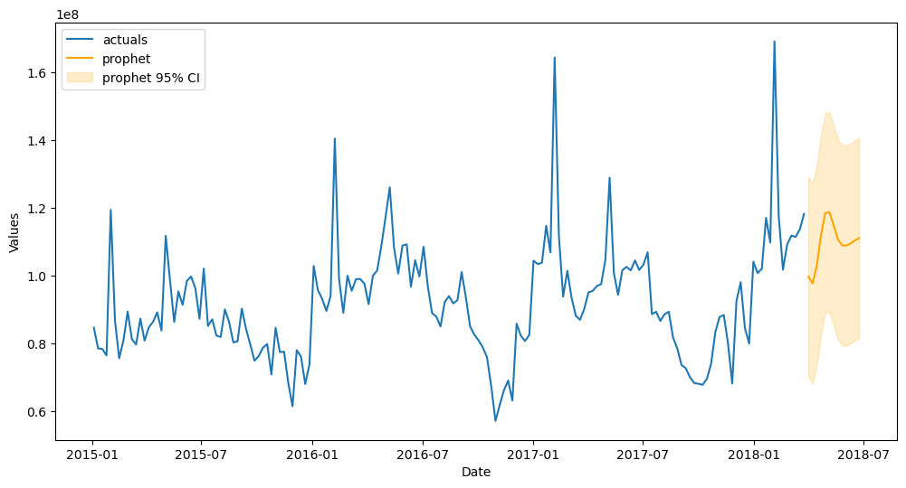
../../_images/misc_introduction_Introduction2_57_0.png

Prophet

[41]:

f.set_estimator('prophet')
f.manual_forecast()

Finished loading model, total used 100 iterations
Finished loading model, total used 100 iterations

22:14:17 - cmdstanpy - INFO - Chain [1] start processing
22:14:17 - cmdstanpy - INFO - Chain [1] done processing
22:14:17 - cmdstanpy - INFO - Chain [1] start processing
22:14:17 - cmdstanpy - INFO - Chain [1] done processing

[42]:

f.plot_test_set(models='prophet',ci=True)
plt.show()

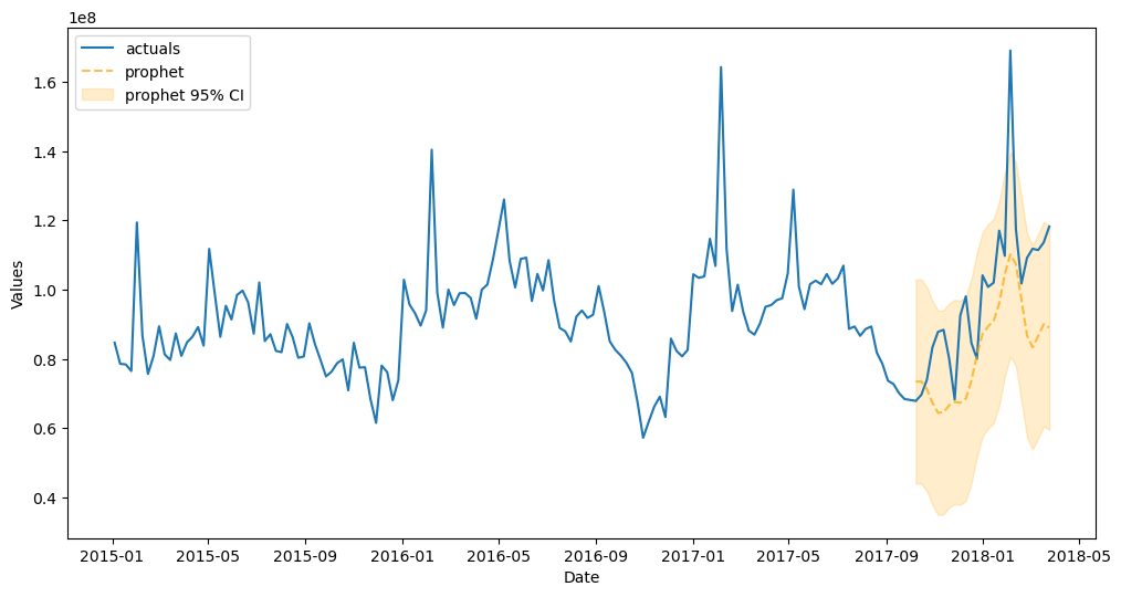
../../_images/misc_introduction_Introduction2_60_0.png

[43]:

f.plot(models='prophet',ci=True)
plt.show()

../../_images/misc_introduction_Introduction2_61_0.png

Other univariate models available: TBATS, Holt-Winters Exponential Smoothing, LSTM, RNN, Silverkite, Theta.

Working on: N-Beats, N-Hits, Genetic Algorithm.

Multivariate Forecasting

Load the `MVForecaster` Object

This object extends the univariate approach to several series, with many of the same plotting and reporting features available.
Documentation

[44]:

from scalecast.MVForecaster import MVForecaster

[45]:

price = data.groupby('Date')['AveragePrice'].mean()

fvol = Forecaster(y=volume,current_dates=volume.index,future_dates=13)
fprice = Forecaster(y=price,current_dates=price.index,future_dates=13)

fvol.add_time_trend()
fvol.add_seasonal_regressors('week',raw=False,sincos=True)

mvf = MVForecaster(
    fvol,
    fprice,
    merge_Xvars='union',
    names=['volume','price'],
)

mvf

[45]:

MVForecaster(
    DateStartActuals=2015-01-04T00:00:00.000000000
    DateEndActuals=2018-03-25T00:00:00.000000000
    Freq=W-SUN
    N_actuals=169
    N_series=2
    SeriesNames=['volume', 'price']
    ForecastLength=13
    Xvars=['t', 'weeksin', 'weekcos']
    TestLength=0
    ValidationLength=1
    ValidationMetric=rmse
    ForecastsEvaluated=[]
    CILevel=None
    CurrentEstimator=mlr
    OptimizeOn=mean
    GridsFile=MVGrids
)

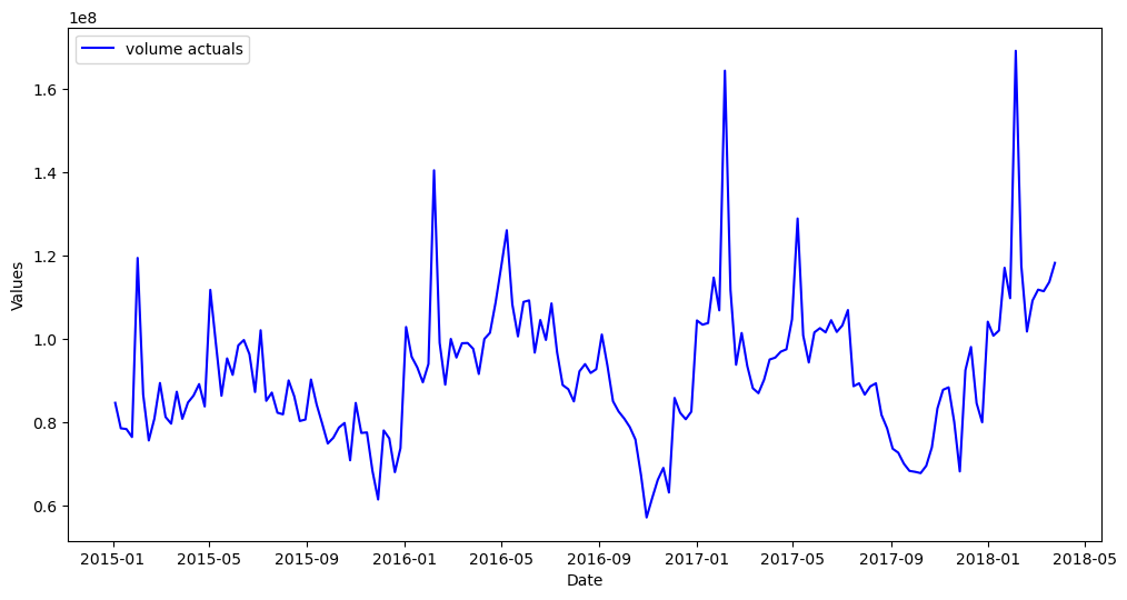
Exploratory Data Analysis

[46]:

mvf.plot(series='volume')
plt.show()

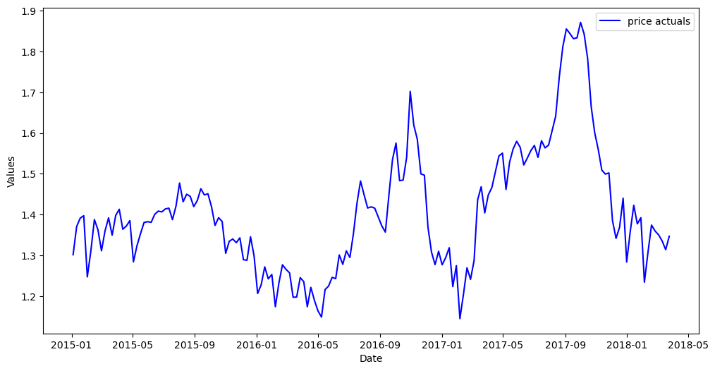
../../_images/misc_introduction_Introduction2_67_0.png

[47]:

mvf.plot(series='price')
plt.show()

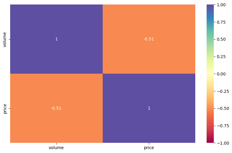
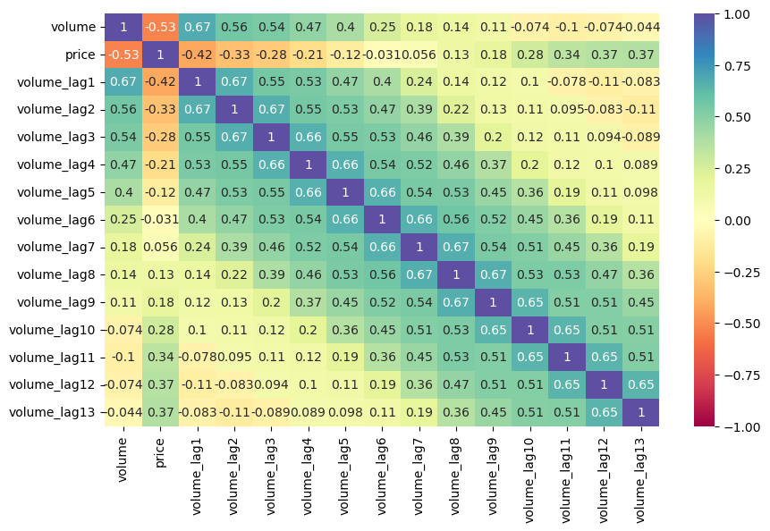
../../_images/misc_introduction_Introduction2_68_0.png

[48]:

mvf.corr(disp='heatmap',cmap='Spectral',annot=True,vmin=-1,vmax=1)
plt.show()

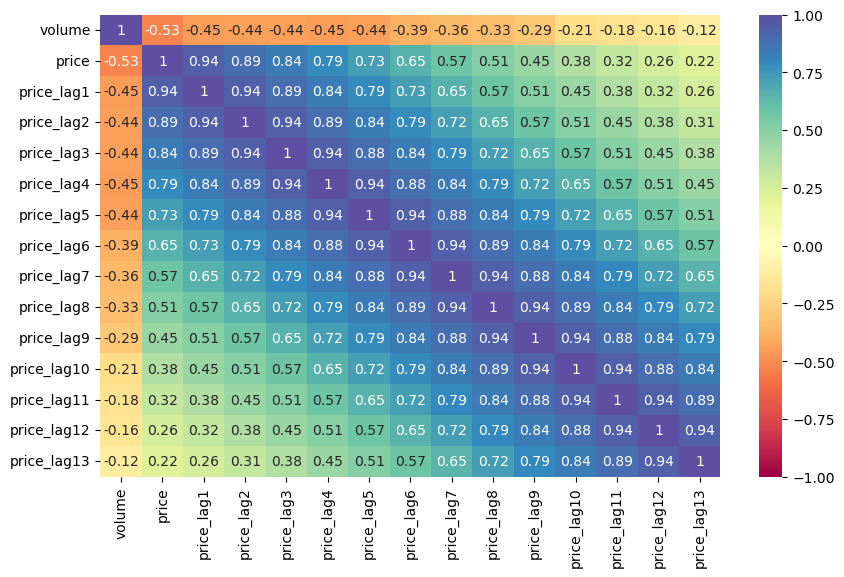
../../_images/misc_introduction_Introduction2_69_0.png

[49]:

mvf.corr_lags(y='price',x='volume',disp='heatmap',cmap='Spectral',annot=True,vmin=-1,vmax=1,lags=13)
plt.show()

../../_images/misc_introduction_Introduction2_70_0.png

[50]:

mvf.corr_lags(y='volume',x='price',disp='heatmap',cmap='Spectral',annot=True,vmin=-1,vmax=1,lags=13)
plt.show()

../../_images/misc_introduction_Introduction2_71_0.png

Parameterize the `MVForecaster` Object

Starting in scalecast version 0.16.0, you can skip model testing by setting a test length of 0.
In this example, all models will be tested on the last 15% of the observed values in the dataset.
We will also have model optimization select hyperparemeters based on what predicts the volume series, rather than the price series, or an average of the two (which is the default), best.
Custom optimization functions are available.

[51]:

mvf.set_test_length(.15)
mvf.set_optimize_on('volume') # we care more about predicting volume and price is just used to make those predictions more accurate
# by default, the optimizer uses an average scoring of all series in the MVForecaster object
mvf.eval_cis() # tell object to evaluate cis

mvf

[51]:

MVForecaster(
    DateStartActuals=2015-01-04T00:00:00.000000000
    DateEndActuals=2018-03-25T00:00:00.000000000
    Freq=W-SUN
    N_actuals=169
    N_series=2
    SeriesNames=['volume', 'price']
    ForecastLength=13
    Xvars=['t', 'weeksin', 'weekcos']
    TestLength=25
    ValidationLength=1
    ValidationMetric=rmse
    ForecastsEvaluated=[]
    CILevel=0.95
    CurrentEstimator=mlr
    OptimizeOn=volume
    GridsFile=MVGrids
)

Run Models

Uses scikit-learn models and APIs only.
See the adapted VECM model for this object.

ElasticNet

[52]:

mvf.set_estimator('elasticnet')
mvf.manual_forecast(alpha=0.2,dynamic_testing=13,lags=13)

XGBoost

[53]:

mvf.set_estimator('xgboost')
mvf.manual_forecast(gamma=1,dynamic_testing=13,lags=13)

MLP Stack

auxmodels.mlp_stack

[54]:

from scalecast.auxmodels import mlp_stack

[55]:

mvf.export('model_summaries')

[55]:

	Series	ModelNickname	Estimator	Xvars	HyperParams	Lags	Observations	DynamicallyTested	TestSetLength	ValidationMetric	ValidationMetricValue	InSampleRMSE	InSampleMAPE	InSampleMAE	InSampleR2	TestSetRMSE	TestSetMAPE	TestSetMAE	TestSetR2
0	volume	elasticnet	elasticnet	[t, weeksin, weekcos]	{'alpha': 0.2}	13	169	13	25	NaN	NaN	1.197603e+07	0.088917	8.206334e+06	0.486109	1.869490e+07	0.118172	1.282436e+07	0.248765
1	volume	xgboost	xgboost	[t, weeksin, weekcos]	{'gamma': 1}	13	169	13	25	NaN	NaN	3.416022e+02	0.000003	2.591667e+02	1.000000	2.260606e+07	0.173554	1.644149e+07	-0.098447
2	price	elasticnet	elasticnet	[t, weeksin, weekcos]	{'alpha': 0.2}	13	169	13	25	NaN	NaN	1.560728e-01	0.084080	1.199107e-01	0.000000	1.522410e-01	0.071282	1.088633e-01	-0.048569
3	price	xgboost	xgboost	[t, weeksin, weekcos]	{'gamma': 1}	13	169	13	25	NaN	NaN	1.141005e-01	0.058215	8.255353e-02	0.465533	1.291758e-01	0.057186	8.791148e-02	0.245089

[56]:

mlp_stack(mvf,model_nicknames=['elasticnet','xgboost'],lags=13)

[57]:

mvf.set_best_model(determine_best_by='TestSetRMSE')

[58]:

mvf.plot_test_set(ci=True,series='volume',put_best_on_top=True)
plt.show()

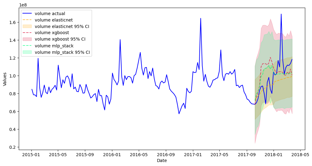
../../_images/misc_introduction_Introduction2_84_0.png

[59]:

mvf.plot(ci=True,series='volume',put_best_on_top=True)
plt.show()

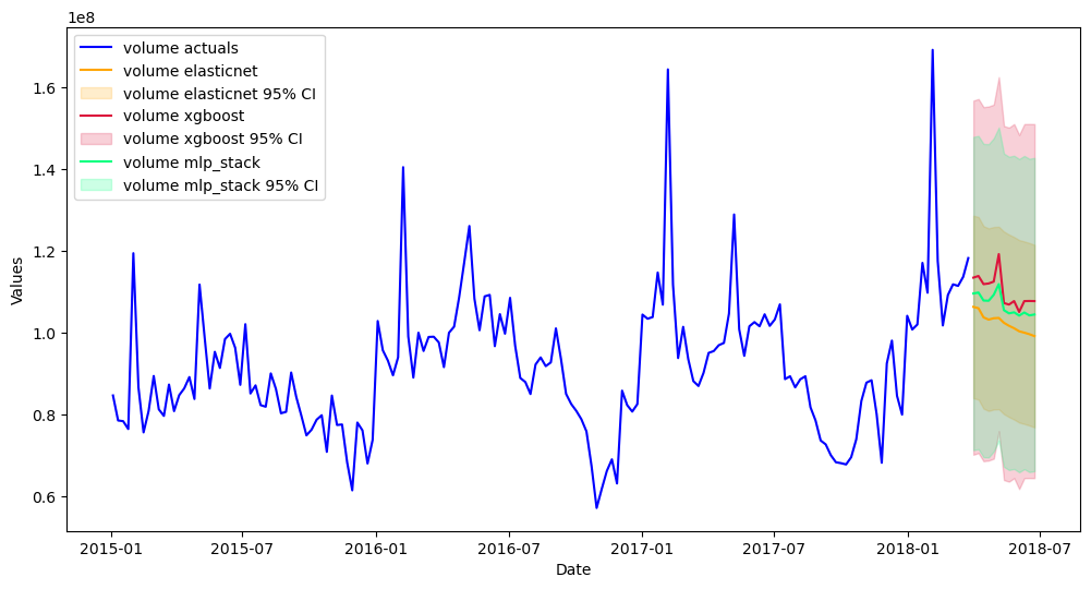
../../_images/misc_introduction_Introduction2_85_0.png

Probabalistic forecasting for creating confidence intervals is currently being worked on in the MVForecaster object, but until that is done, the backtested interval also works well:

[60]:

mvf.plot(ci=True,series='volume',put_best_on_top=True)
plt.show()

../../_images/misc_introduction_Introduction2_87_0.png

Break Back into Forecaster Objects

You can then add univariate models to these objects to compare with the models run multivariate.

[61]:

from scalecast.util import break_mv_forecaster

[62]:

fvol, fprice = break_mv_forecaster(mvf)

[63]:

fvol

[63]:

Forecaster(
    DateStartActuals=2015-01-04T00:00:00.000000000
    DateEndActuals=2018-03-25T00:00:00.000000000
    Freq=W-SUN
    N_actuals=169
    ForecastLength=13
    Xvars=[]
    TestLength=25
    ValidationMetric=rmse
    ForecastsEvaluated=['elasticnet', 'xgboost', 'mlp_stack']
    CILevel=0.95
    CurrentEstimator=mlr
    GridsFile=Grids
)

[64]:

fprice

[64]:

Forecaster(
    DateStartActuals=2015-01-04T00:00:00.000000000
    DateEndActuals=2018-03-25T00:00:00.000000000
    Freq=W-SUN
    N_actuals=169
    ForecastLength=13
    Xvars=[]
    TestLength=25
    ValidationMetric=rmse
    ForecastsEvaluated=['elasticnet', 'xgboost', 'mlp_stack']
    CILevel=0.95
    CurrentEstimator=mlr
    GridsFile=Grids
)

Transformations

One of the most effective way to boost forecasting power is with transformations.
Transformations include:
Log
Scaling
- Standard
- MinMax
Differencing
Detrending
Custom Functions
All transformations have a corresponding revert function.
See the blog post.

[65]:

from scalecast.SeriesTransformer import SeriesTransformer

[66]:

f_trans = Forecaster(y=volume,current_dates=volume.index,future_dates=13)

[67]:

f_trans.set_test_length(.15)
f_trans.set_validation_length(13)

[68]:

transformer = SeriesTransformer(f_trans)

[69]:

# these will all be reverted later after forecasts have been called
f_trans = transformer.DiffTransform(1)
f_trans = transformer.DiffTransform(52)
f_trans = transformer.DetrendTransform()

[70]:

f_trans.plot()
plt.show()

../../_images/misc_introduction_Introduction2_99_0.png

[71]:

f_trans.add_time_trend()
f_trans.add_seasonal_regressors('week',sincos=True,raw=False)
f_trans.add_ar_terms(13)

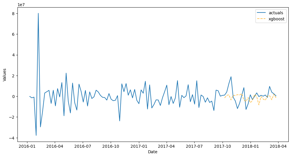
[72]:

f_trans.set_estimator('xgboost')
f_trans.manual_forecast(gamma=1,dynamic_testing=13)

[73]:

f_trans.plot_test_set()
plt.show()

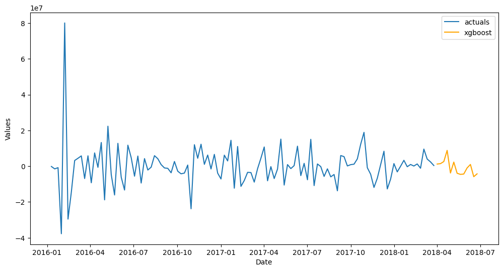
../../_images/misc_introduction_Introduction2_102_0.png

[74]:

f_trans.plot()
plt.show()

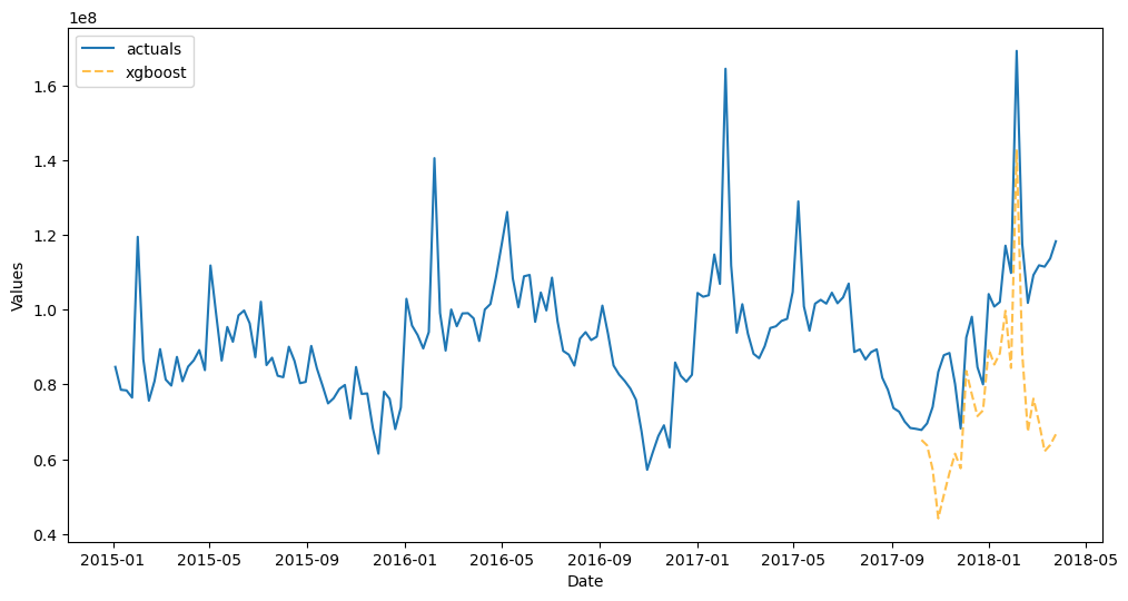
../../_images/misc_introduction_Introduction2_103_0.png

[75]:

# call revert functions in the opposite order as how they were called when transforming
f_trans = transformer.DetrendRevert()
f_trans = transformer.DiffRevert(52)
f_trans = transformer.DiffRevert(1)

[76]:

f_trans.plot_test_set()
plt.show()

../../_images/misc_introduction_Introduction2_105_0.png

[77]:

f_trans.plot()
plt.show()

../../_images/misc_introduction_Introduction2_106_0.png

Pipelines

These are objects similar to scikit-learn pipelines that offer readable and streamlined code for transforming, forecasting, and reverting.
See the Pipeline object documentation.

[78]:

from scalecast.Pipeline import Transformer, Reverter, Pipeline, MVPipeline

[79]:

f_pipe = Forecaster(y=volume,current_dates=volume.index,future_dates=13)
f_pipe.set_test_length(.15)

[80]:

def forecaster(f):
    f.add_time_trend()
    f.add_seasonal_regressors('week',raw=False,sincos=True)
    f.add_ar_terms(13)
    f.set_estimator('lightgbm')
    f.manual_forecast(max_depth=2)

[81]:

transformer = Transformer(
    transformers = [
        ('DiffTransform',1),
        ('DiffTransform',52),
        ('DetrendTransform',)
    ]
)

reverter = Reverter(
    reverters = [
        ('DetrendRevert',),
        ('DiffRevert',52),
        ('DiffRevert',1)
    ],
    base_transformer = transformer,
)

[82]:

reverter

[82]:

Reverter(
  reverters = [
    ('DetrendRevert',),
    ('DiffRevert', 52),
    ('DiffRevert', 1)
  ],
  base_transformer = Transformer(
  transformers = [
    ('DiffTransform', 1),
    ('DiffTransform', 52),
    ('DetrendTransform',)
  ]
)
)

[83]:

pipeline = Pipeline(
    steps = [
        ('Transform',transformer),
        ('Forecast',forecaster),
        ('Revert',reverter),
    ]
)

f_pipe = pipeline.fit_predict(f_pipe)

[84]:

f_pipe.plot_test_set()
plt.show()

../../_images/misc_introduction_Introduction2_114_0.png

[85]:

f_pipe.plot()
plt.show()

../../_images/misc_introduction_Introduction2_115_0.png

Fully Automated Pipelines

We can automate the construction of pipelines, the selection of input variables, and tuning of models with cross validation on a grid search for each model using files in the working directory called Grids.py for univariate forecasting and MVGrids.py for multivariate. Default grids can be downloaded from scalecast.

Automated Univariate Pipelines

Documentation

[86]:

from scalecast import GridGenerator
from scalecast.util import find_optimal_transformation

[87]:

GridGenerator.get_example_grids(overwrite=True)

[88]:

f_pipe_aut = Forecaster(y=volume,current_dates=volume.index,future_dates=13)
f_pipe_aut.set_test_length(.15)

[89]:

def forecaster_aut(f,models):
    f.auto_Xvar_select(
        estimator='elasticnet',
        monitor='TestSetMAE',
        alpha=0.2,
        irr_cycles = [26],
    )
    f.tune_test_forecast(
        models,
        cross_validate=True,
        k=3,
        # dynamic tuning = 13 means we will hopefully find a model that is optimized to predict 13 steps
        dynamic_tuning=13,
        dynamic_testing=13,
    )
    f.set_estimator('combo')
    f.manual_forecast()

util.find_optimal_transformation

In this function, the following transformations are searched for:
- Detrending
- Box-Cox
- First Differencing
- Seasonal Differencing
- Scaling

The optimal set of transformations are returned based on best estimated out-of-sample performance on the test set. Therefore, running this function introduces leakage into the test set, but it can still be a good addition to an automated pipeline, depending on the application. Which and the order of transfomations to search through are configurable. How performance is measured, the parameters specific to a given transformation, and several other paramters are also configurable. See the documentation.

[90]:

transformer_aut, reverter_aut = find_optimal_transformation(
    f_pipe_aut,
    lags = 13,
    m = 52,
    monitor = 'mae',
    estimator = 'elasticnet',
    alpha = 0.2,
    test_length = 13,
    num_test_sets = 3,
    space_between_sets = 4,
    verbose = True,
) # returns a Transformer and Reverter object that can be plugged into a larger pipeline

All transformation tries will use 13 lags.
Last transformer tried:
[]
Score (mae): 17933061.20374991
--------------------------------------------------
Last transformer tried:
[('DetrendTransform', {'loess': True})]
Score (mae): 23964157.165726673
--------------------------------------------------
Last transformer tried:
[('DetrendTransform', {'poly_order': 1})]
Score (mae): 17174376.36667074
--------------------------------------------------
Last transformer tried:
[('DetrendTransform', {'poly_order': 2})]
Score (mae): 24467364.037868027
--------------------------------------------------
Last transformer tried:
[('DetrendTransform', {'poly_order': 1}), ('DeseasonTransform', {'m': 52, 'model': 'add'})]
Score (mae): 11573053.425807403
--------------------------------------------------
Last transformer tried:
[('DetrendTransform', {'poly_order': 1}), ('DeseasonTransform', {'m': 52, 'model': 'add'}), ('DiffTransform', 1)]
Score (mae): 9478522.651025781
--------------------------------------------------
Last transformer tried:
[('DetrendTransform', {'poly_order': 1}), ('DeseasonTransform', {'m': 52, 'model': 'add'}), ('DiffTransform', 1), ('DiffTransform', 52)]
Score (mae): 11116081.856823219
--------------------------------------------------
Last transformer tried:
[('DetrendTransform', {'poly_order': 1}), ('DeseasonTransform', {'m': 52, 'model': 'add'}), ('DiffTransform', 1), ('ScaleTransform',)]
Score (mae): 9583504.942193026
--------------------------------------------------
Last transformer tried:
[('DetrendTransform', {'poly_order': 1}), ('DeseasonTransform', {'m': 52, 'model': 'add'}), ('DiffTransform', 1), ('MinMaxTransform',)]
Score (mae): 9583504.942193048
--------------------------------------------------
Final Selection:
[('DetrendTransform', {'poly_order': 1}), ('DeseasonTransform', {'m': 52, 'model': 'add'}), ('DiffTransform', 1)]

[91]:

pipeline_aut = Pipeline(
    steps = [
        ('Transform',transformer_aut),
        ('Forecast',forecaster_aut),
        ('Revert',reverter_aut),
    ]
)

f_pipe_aut = pipeline_aut.fit_predict(
    f_pipe_aut,
    models=[
        'mlr',
        'elasticnet',
        'xgboost',
        'lightgbm',
        'knn',
    ],
)

Finished loading model, total used 200 iterations
Finished loading model, total used 200 iterations
Finished loading model, total used 200 iterations
Finished loading model, total used 200 iterations
Finished loading model, total used 200 iterations

[92]:

f_pipe_aut

[92]:

Forecaster(
    DateStartActuals=2015-01-04T00:00:00.000000000
    DateEndActuals=2018-03-25T00:00:00.000000000
    Freq=W-SUN
    N_actuals=169
    ForecastLength=13
    Xvars=['AR1', 'AR2', 'AR3', 'AR4', 'AR5']
    TestLength=25
    ValidationMetric=rmse
    ForecastsEvaluated=['mlr', 'elasticnet', 'xgboost', 'lightgbm', 'knn', 'combo']
    CILevel=None
    CurrentEstimator=combo
    GridsFile=Grids
)

[93]:

f_pipe_aut.plot_test_set(order_by='TestSetRMSE')
plt.show()

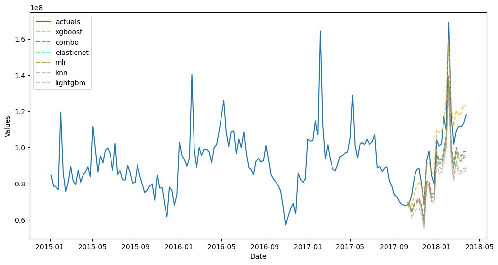
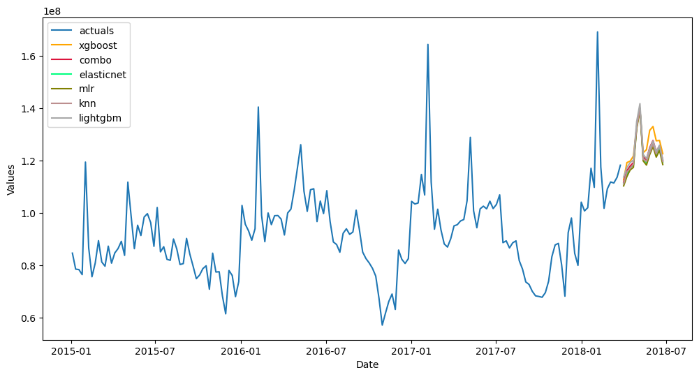
../../_images/misc_introduction_Introduction2_126_0.png

[94]:

f_pipe_aut.plot(order_by='TestSetRMSE')
plt.show()

../../_images/misc_introduction_Introduction2_127_0.png

Backtest Univariate Pipeline

You may be interested to know beyond a single test-set metric, how well your pipeline performs out-of-sample. Backtesting can help answer that by iterating through the entire pipeline several times and testing the procedure each time. It can also help make expanding confidence intervals. See the documentation.

[95]:

from scalecast.util import backtest_metrics

[96]:

uv_backtest_results = pipeline_aut.backtest(
    f_pipe_aut,
    n_iter = 3,
    jump_back = 13,
    cis = False,
    models=[
        'mlr',
        'elasticnet',
        'xgboost',
        'lightgbm',
        'knn',
    ],
)

Finished loading model, total used 150 iterations
Finished loading model, total used 150 iterations
Finished loading model, total used 150 iterations
Finished loading model, total used 150 iterations
Finished loading model, total used 150 iterations
Finished loading model, total used 200 iterations
Finished loading model, total used 200 iterations
Finished loading model, total used 200 iterations
Finished loading model, total used 200 iterations
Finished loading model, total used 200 iterations
Finished loading model, total used 200 iterations
Finished loading model, total used 200 iterations
Finished loading model, total used 200 iterations
Finished loading model, total used 200 iterations
Finished loading model, total used 200 iterations

After obtaining the results from the backtest, we can see the average performance over each iteration using the util.backtest_metrics function. See the documentation.

[97]:

pd.options.display.float_format = '{:,.4f}'.format
backtest_metrics(
    uv_backtest_results,
    mets=['smape','rmse','bias'],
)

[97]:

		Iter0	Iter1	Iter2	Average
Model	Metric
mlr	smape	0.1130	0.2317	0.1142	0.1529
	rmse	15,488,744.6687	19,538,227.8483	11,910,709.6300	15,645,894.0490
	bias	-165,115,026.5519	-207,268,257.9313	103,757,419.4097	-89,541,955.0245
elasticnet	smape	0.1237	0.1962	0.1428	0.1542
	rmse	16,732,592.7781	16,625,313.2954	14,338,412.2989	15,898,772.7908
	bias	-177,765,519.3932	-169,974,287.0231	145,808,728.0805	-67,310,359.4453
xgboost	smape	0.0978	0.2221	0.1710	0.1636
	rmse	13,607,549.8360	18,573,088.5135	18,136,645.4700	16,772,427.9399
	bias	-139,025,946.3310	-187,065,120.1406	180,813,791.1197	-48,425,758.4506
lightgbm	smape	0.1248	0.2178	0.1483	0.1636
	rmse	16,803,405.5145	18,415,746.1087	15,074,267.8093	16,764,473.1442
	bias	-176,880,323.1388	-195,683,280.2443	149,272,223.4129	-74,430,459.9901
knn	smape	0.2044	0.1896	0.1439	0.1793
	rmse	23,802,323.7447	16,441,684.0561	14,418,665.8740	18,220,891.2249
	bias	-278,780,122.9043	-174,089,027.5994	145,204,593.3703	-102,554,852.3778
combo	smape	0.1304	0.2109	0.1438	0.1617
	rmse	17,124,663.5858	17,869,415.4842	14,723,986.4866	16,572,688.5189
	bias	-187,513,387.6638	-186,815,994.5877	144,971,351.0786	-76,452,677.0576

Automated Multivariate Pipelines

See the MVPipeline object documentation.

[98]:

GridGenerator.get_mv_grids(overwrite=True)

[99]:

fvol_aut = Forecaster(
    y=volume,
    current_dates=volume.index,
    future_dates=13,
    test_length = .15,
)
fprice_aut = Forecaster(
    y=price,
    current_dates=price.index,
    future_dates=13,
    test_length = .15,
)

[100]:

def add_vars(f,**kwargs):
    f.add_seasonal_regressors(
        'month',
        'quarter',
        'week',
        raw=False,
        sincos=True
    )

def mvforecaster(mvf,models):
    mvf.set_optimize_on('volume')
    mvf.tune_test_forecast(
        models,
        cross_validate=True,
        k=2,
        rolling=True,
        dynamic_tuning=13,
        dynamic_testing=13,
        limit_grid_size = .2,
        error = 'warn',
    )

[101]:

transformer_vol, reverter_vol = find_optimal_transformation(
    fvol_aut,
    lags = 13,
    m = 52,
    monitor = 'mae',
    estimator = 'elasticnet',
    alpha = 0.2,
    test_length = 13,
    num_test_sets = 3,
    space_between_sets = 4,
    verbose = True,
)

All transformation tries will use 13 lags.
Last transformer tried:
[]
Score (mae): 17933061.20374991
--------------------------------------------------
Last transformer tried:
[('DetrendTransform', {'loess': True})]
Score (mae): 23964157.165726673
--------------------------------------------------
Last transformer tried:
[('DetrendTransform', {'poly_order': 1})]
Score (mae): 17174376.36667074
--------------------------------------------------
Last transformer tried:
[('DetrendTransform', {'poly_order': 2})]
Score (mae): 24467364.037868027
--------------------------------------------------
Last transformer tried:
[('DetrendTransform', {'poly_order': 1}), ('DeseasonTransform', {'m': 52, 'model': 'add'})]
Score (mae): 11573053.425807403
--------------------------------------------------
Last transformer tried:
[('DetrendTransform', {'poly_order': 1}), ('DeseasonTransform', {'m': 52, 'model': 'add'}), ('DiffTransform', 1)]
Score (mae): 9478522.651025781
--------------------------------------------------
Last transformer tried:
[('DetrendTransform', {'poly_order': 1}), ('DeseasonTransform', {'m': 52, 'model': 'add'}), ('DiffTransform', 1), ('DiffTransform', 52)]
Score (mae): 11116081.856823219
--------------------------------------------------
Last transformer tried:
[('DetrendTransform', {'poly_order': 1}), ('DeseasonTransform', {'m': 52, 'model': 'add'}), ('DiffTransform', 1), ('ScaleTransform',)]
Score (mae): 9583504.942193026
--------------------------------------------------
Last transformer tried:
[('DetrendTransform', {'poly_order': 1}), ('DeseasonTransform', {'m': 52, 'model': 'add'}), ('DiffTransform', 1), ('MinMaxTransform',)]
Score (mae): 9583504.942193048
--------------------------------------------------
Final Selection:
[('DetrendTransform', {'poly_order': 1}), ('DeseasonTransform', {'m': 52, 'model': 'add'}), ('DiffTransform', 1)]

[102]:

transformer_price, reverter_price = find_optimal_transformation(
    fprice_aut,
    lags = 13,
    m = 52,
    monitor = 'mae',
    estimator = 'elasticnet',
    alpha = 0.2,
    test_length = 13,
    num_test_sets = 3,
    space_between_sets = 4,
    verbose = True,
)

All transformation tries will use 13 lags.
Last transformer tried:
[]
Score (mae): 0.06804292152560591
--------------------------------------------------
Last transformer tried:
[('DetrendTransform', {'loess': True})]
Score (mae): 0.35311292233215247
--------------------------------------------------
Last transformer tried:
[('DetrendTransform', {'poly_order': 1})]
Score (mae): 0.18654572266988656
--------------------------------------------------
Last transformer tried:
[('DetrendTransform', {'poly_order': 2})]
Score (mae): 0.407907120834863
--------------------------------------------------
Last transformer tried:
[('DeseasonTransform', {'m': 52, 'model': 'add'})]
Score (mae): 0.04226554848615107
--------------------------------------------------
Last transformer tried:
[('DeseasonTransform', {'m': 52, 'model': 'add'}), ('Transform', <function find_optimal_transformation.<locals>.boxcox_tr at 0x7fcff088d040>, {'lmbda': -0.5})]
Score (mae): 0.047544210787943963
--------------------------------------------------
Last transformer tried:
[('DeseasonTransform', {'m': 52, 'model': 'add'}), ('Transform', <function find_optimal_transformation.<locals>.boxcox_tr at 0x7fcff088d040>, {'lmbda': 0})]
Score (mae): 0.04573807786929981
--------------------------------------------------
Last transformer tried:
[('DeseasonTransform', {'m': 52, 'model': 'add'}), ('Transform', <function find_optimal_transformation.<locals>.boxcox_tr at 0x7fcff088d040>, {'lmbda': 0.5})]
Score (mae): 0.04392809054109548
--------------------------------------------------
Last transformer tried:
[('DeseasonTransform', {'m': 52, 'model': 'add'}), ('DiffTransform', 1)]
Score (mae): 0.08609820028223651
--------------------------------------------------
Last transformer tried:
[('DeseasonTransform', {'m': 52, 'model': 'add'}), ('DiffTransform', 52)]
Score (mae): 0.05863628346364504
--------------------------------------------------
Last transformer tried:
[('DeseasonTransform', {'m': 52, 'model': 'add'}), ('ScaleTransform',)]
Score (mae): 0.038603715602285725
--------------------------------------------------
Last transformer tried:
[('DeseasonTransform', {'m': 52, 'model': 'add'}), ('MinMaxTransform',)]
Score (mae): 0.042265548486150994
--------------------------------------------------
Final Selection:
[('DeseasonTransform', {'m': 52, 'model': 'add'}), ('ScaleTransform',)]

[103]:

mvpipeline = MVPipeline(
    steps = [
        ('Transform',[transformer_vol,transformer_price]),
        ('Add Xvars',[add_vars]*2),
        ('Forecast',mvforecaster),
        ('Revert',[reverter_vol,reverter_price]),
    ],
    test_length = 20,
    cis = True,
    names = ['volume','price'],
)

fvol_aut, fprice_aut = mvpipeline.fit_predict(
    fvol_aut,
    fprice_aut,
    models=[
        'mlr',
        'elasticnet',
        'xgboost',
        'lightgbm',
    ],
) # returns a tuple of Forecaster objects

Finished loading model, total used 200 iterations
Finished loading model, total used 200 iterations

[104]:

fvol_aut.plot_test_set(order_by='TestSetRMSE',ci=True)
plt.show()

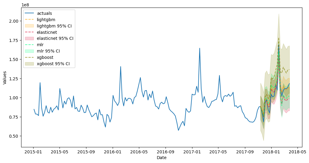
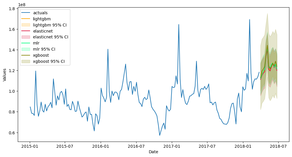
../../_images/misc_introduction_Introduction2_140_0.png

[105]:

fvol_aut.plot(order_by='TestSetRMSE',ci=True)
plt.show()

../../_images/misc_introduction_Introduction2_141_0.png

Backtest Multivariate Pipeline

Like univariate pipelines, multivariate pipelines can also be backtested. Info about each model and series becomes possible to compare. See the documentation.

[106]:

# recreate Forecaster objects to bring dates back lost from taking seasonal differences
fvol_aut = Forecaster(
    y=volume,
    current_dates=volume.index,
    future_dates=13,
)
fprice_aut = Forecaster(
    y=price,
    current_dates=price.index,
    future_dates=13,
)

[107]:

mv_backtest_results = mvpipeline.backtest(
    fvol_aut,
    fprice_aut,
    n_iter = 3,
    jump_back = 13,
    test_length = 0,
    cis = False,
    models=[
        'mlr',
        'elasticnet',
        'xgboost',
        'lightgbm',
    ],
)

Finished loading model, total used 250 iterations
Finished loading model, total used 250 iterations
Finished loading model, total used 200 iterations
Finished loading model, total used 200 iterations
Finished loading model, total used 250 iterations
Finished loading model, total used 250 iterations

[108]:

backtest_metrics(
    mv_backtest_results,
    mets=['smape','rmse','bias'],
    names = ['Volume','Price'],
)

[108]:

			Iter0	Iter1	Iter2	Average
Series	Model	Metric
Volume	mlr	smape	0.0544	0.1176	0.1582	0.1101
		rmse	9,607,094.0997	10,760,756.5379	15,963,833.7533	12,110,561.4636
		bias	-69,742,732.2916	-87,711,912.6597	157,394,405.8767	-20,079.6915
	elasticnet	smape	0.0662	0.1606	0.1398	0.1222
		rmse	10,759,298.7685	14,132,016.6443	14,134,913.2323	13,008,742.8817
		bias	-82,997,021.2184	-139,537,507.0051	140,719,790.4827	-27,271,579.2469
	xgboost	smape	0.1315	0.1447	0.0713	0.1158
		rmse	20,090,059.9856	13,817,186.7925	7,510,114.4244	13,805,787.0675
		bias	189,709,643.4190	-129,669,530.7265	71,329,272.6822	43,789,795.1249
	lightgbm	smape	0.1278	0.1161	0.1720	0.1386
		rmse	16,974,627.6371	10,539,060.5819	17,427,536.4398	14,980,408.2196
		bias	-182,115,273.5654	-76,693,584.9027	184,015,627.3148	-24,931,077.0511
Price	mlr	smape	0.0523	0.0762	0.0808	0.0698
		rmse	0.0811	0.1307	0.1782	0.1300
		bias	0.9321	1.0663	-1.5867	0.1372
	elasticnet	smape	0.0287	0.0606	0.1631	0.0841
		rmse	0.0461	0.1043	0.2838	0.1447
		bias	-0.1421	0.5670	-3.3627	-0.9793
	xgboost	smape	0.0656	0.0513	0.1053	0.0740
		rmse	0.1000	0.1024	0.2100	0.1375
		bias	1.1779	0.1599	-2.2494	-0.3038
	lightgbm	smape	0.0287	0.0630	0.1588	0.0835
		rmse	0.0459	0.1215	0.2799	0.1491
		bias	-0.2103	-0.1697	-3.2847	-1.2215

Through backtesting, we can see that the multivariate approach out-performed the univariate approach. Very cool!

Scaled Automated Forecasting

We can scale the fully automated approach to many series where we can then access all results through plotting with Jupyter widgets and export functions.
We produce a separate forecast for avocado sales in each region in our dataset.
This is done with a univariate approach, but cleverly using the code in this notebook, it could be transformed into a multivariate process where volume and price are forecasted together.

[109]:

from scalecast.notebook import results_vis
from tqdm.notebook import tqdm

[110]:

def forecaster_scaled(f,models):
    f.auto_Xvar_select(
        estimator='elasticnet',
        monitor='TestSetMAE',
        alpha=0.2,
        irr_cycles = [26],
    )
    f.tune_test_forecast(
        models,
        dynamic_testing=13,
    )
    f.set_estimator('combo')
    f.manual_forecast()

[111]:

results_dict = {}
for region in tqdm(data.region.unique()):
    series = data.loc[data['region'] == region].groupby('Date')['Total Volume'].sum()
    f_i = Forecaster(
        y = series,
        current_dates = series.index,
        future_dates = 13,
        test_length = .15,
        validation_length = 13,
        cis = True,
    )
    transformer_i, reverter_i = find_optimal_transformation(
        f_i,
        lags = 13,
        m = 52,
        monitor = 'mae',
        estimator = 'elasticnet',
        alpha = 0.2,
        test_length = 13,
    )
    pipeline_i = Pipeline(
        steps = [
            ('Transform',transformer_i),
            ('Forecast',forecaster_scaled),
            ('Revert',reverter_i),
        ]
    )
    f_i = pipeline_i.fit_predict(
        f_i,
        models=[
            'mlr',
            'elasticnet',
            'xgboost',
            'lightgbm',
            'knn',
        ],
    )
    results_dict[region] = f_i

Finished loading model, total used 250 iterations
Finished loading model, total used 250 iterations
Finished loading model, total used 250 iterations
Finished loading model, total used 150 iterations
Finished loading model, total used 150 iterations
Finished loading model, total used 150 iterations
Finished loading model, total used 150 iterations
Finished loading model, total used 150 iterations
Finished loading model, total used 150 iterations
Finished loading model, total used 250 iterations
Finished loading model, total used 250 iterations
Finished loading model, total used 250 iterations
Finished loading model, total used 150 iterations
Finished loading model, total used 150 iterations
Finished loading model, total used 150 iterations
Finished loading model, total used 200 iterations
Finished loading model, total used 200 iterations
Finished loading model, total used 200 iterations
Finished loading model, total used 150 iterations
Finished loading model, total used 150 iterations
Finished loading model, total used 150 iterations
Finished loading model, total used 150 iterations
Finished loading model, total used 150 iterations
Finished loading model, total used 150 iterations
Finished loading model, total used 150 iterations
Finished loading model, total used 150 iterations
Finished loading model, total used 150 iterations
Finished loading model, total used 150 iterations
Finished loading model, total used 150 iterations
Finished loading model, total used 150 iterations
Finished loading model, total used 200 iterations
Finished loading model, total used 200 iterations
Finished loading model, total used 200 iterations
Finished loading model, total used 250 iterations
Finished loading model, total used 250 iterations
Finished loading model, total used 250 iterations
Finished loading model, total used 150 iterations
Finished loading model, total used 150 iterations
Finished loading model, total used 150 iterations
Finished loading model, total used 150 iterations
Finished loading model, total used 150 iterations
Finished loading model, total used 150 iterations
Finished loading model, total used 250 iterations
Finished loading model, total used 250 iterations
Finished loading model, total used 250 iterations
Finished loading model, total used 250 iterations
Finished loading model, total used 250 iterations
Finished loading model, total used 250 iterations
Finished loading model, total used 150 iterations
Finished loading model, total used 150 iterations
Finished loading model, total used 150 iterations
Finished loading model, total used 250 iterations
Finished loading model, total used 250 iterations
Finished loading model, total used 250 iterations
Finished loading model, total used 150 iterations
Finished loading model, total used 150 iterations
Finished loading model, total used 150 iterations
Finished loading model, total used 150 iterations
Finished loading model, total used 150 iterations
Finished loading model, total used 150 iterations
Finished loading model, total used 150 iterations
Finished loading model, total used 150 iterations
Finished loading model, total used 150 iterations
Finished loading model, total used 200 iterations
Finished loading model, total used 200 iterations
Finished loading model, total used 200 iterations
Finished loading model, total used 150 iterations
Finished loading model, total used 150 iterations
Finished loading model, total used 150 iterations
Finished loading model, total used 150 iterations
Finished loading model, total used 150 iterations
Finished loading model, total used 150 iterations
Finished loading model, total used 250 iterations
Finished loading model, total used 250 iterations
Finished loading model, total used 250 iterations
Finished loading model, total used 150 iterations
Finished loading model, total used 150 iterations
Finished loading model, total used 150 iterations
Finished loading model, total used 10 iterations
Finished loading model, total used 10 iterations
Finished loading model, total used 10 iterations
Finished loading model, total used 250 iterations
Finished loading model, total used 250 iterations
Finished loading model, total used 250 iterations
Finished loading model, total used 150 iterations
Finished loading model, total used 150 iterations
Finished loading model, total used 150 iterations
Finished loading model, total used 150 iterations
Finished loading model, total used 150 iterations
Finished loading model, total used 150 iterations
Finished loading model, total used 150 iterations
Finished loading model, total used 150 iterations
Finished loading model, total used 150 iterations
Finished loading model, total used 150 iterations
Finished loading model, total used 150 iterations
Finished loading model, total used 150 iterations
Finished loading model, total used 150 iterations
Finished loading model, total used 150 iterations
Finished loading model, total used 150 iterations
Finished loading model, total used 200 iterations
Finished loading model, total used 200 iterations
Finished loading model, total used 200 iterations
Finished loading model, total used 150 iterations
Finished loading model, total used 150 iterations
Finished loading model, total used 150 iterations
Finished loading model, total used 250 iterations
Finished loading model, total used 250 iterations
Finished loading model, total used 250 iterations
Finished loading model, total used 250 iterations
Finished loading model, total used 250 iterations
Finished loading model, total used 250 iterations
Finished loading model, total used 100 iterations
Finished loading model, total used 100 iterations
Finished loading model, total used 100 iterations
Finished loading model, total used 150 iterations
Finished loading model, total used 150 iterations
Finished loading model, total used 150 iterations
Finished loading model, total used 250 iterations
Finished loading model, total used 250 iterations
Finished loading model, total used 250 iterations
Finished loading model, total used 250 iterations
Finished loading model, total used 250 iterations
Finished loading model, total used 250 iterations
Finished loading model, total used 150 iterations
Finished loading model, total used 150 iterations
Finished loading model, total used 150 iterations
Finished loading model, total used 150 iterations
Finished loading model, total used 150 iterations
Finished loading model, total used 150 iterations
Finished loading model, total used 150 iterations
Finished loading model, total used 150 iterations
Finished loading model, total used 150 iterations
Finished loading model, total used 250 iterations
Finished loading model, total used 250 iterations
Finished loading model, total used 250 iterations
Finished loading model, total used 150 iterations
Finished loading model, total used 150 iterations
Finished loading model, total used 150 iterations
Finished loading model, total used 150 iterations
Finished loading model, total used 150 iterations
Finished loading model, total used 150 iterations
Finished loading model, total used 250 iterations
Finished loading model, total used 250 iterations
Finished loading model, total used 250 iterations
Finished loading model, total used 250 iterations
Finished loading model, total used 250 iterations
Finished loading model, total used 250 iterations
Finished loading model, total used 250 iterations
Finished loading model, total used 250 iterations
Finished loading model, total used 250 iterations
Finished loading model, total used 250 iterations
Finished loading model, total used 250 iterations
Finished loading model, total used 250 iterations
Finished loading model, total used 250 iterations
Finished loading model, total used 250 iterations
Finished loading model, total used 250 iterations
Finished loading model, total used 250 iterations
Finished loading model, total used 250 iterations
Finished loading model, total used 250 iterations
Finished loading model, total used 250 iterations
Finished loading model, total used 250 iterations
Finished loading model, total used 250 iterations

Run the next two functions locally to see the full functionality of these widgets.

[112]:

results_vis(results_dict,'test')

[113]:

results_vis(results_dict)

Exporting Results

[114]:

from scalecast.multiseries import export_model_summaries

Exporting Results from a Single `Forecaster` Object

[115]:

results = f.export(cis=True,models=['mlr','lasso','ridge'])
results.keys()

[115]:

dict_keys(['model_summaries', 'lvl_fcsts', 'lvl_test_set_predictions'])

[116]:

for k, df in results.items():
    print(f'{k} has these columns:',*df.columns,'-'*25,sep='\n')

model_summaries has these columns:
ModelNickname
Estimator
Xvars
HyperParams
Observations
DynamicallyTested
TestSetLength
CILevel
ValidationMetric
ValidationMetricValue
models
weights
best_model
InSampleRMSE
InSampleMAPE
InSampleMAE
InSampleR2
TestSetRMSE
TestSetMAPE
TestSetMAE
TestSetR2
-------------------------
lvl_fcsts has these columns:
DATE
mlr
mlr_upperci
mlr_lowerci
lasso
lasso_upperci
lasso_lowerci
ridge
ridge_upperci
ridge_lowerci
-------------------------
lvl_test_set_predictions has these columns:
DATE
actual
mlr
mlr_upperci
mlr_lowerci
lasso
lasso_upperci
lasso_lowerci
ridge
ridge_upperci
ridge_lowerci
-------------------------

[117]:

results['model_summaries'][['ModelNickname','HyperParams','TestSetRMSE','InSampleRMSE']]

[117]:

	ModelNickname	HyperParams	TestSetRMSE	InSampleRMSE
0	mlr	{}	16,818,489.5277	10,231,495.9303
1	lasso	{'alpha': 0.2}	16,818,489.9828	10,231,495.9303
2	ridge	{'alpha': 0.2}	16,827,165.4875	10,265,352.0145

Other export functions:
Forecaster.export_Xvars_df
Forecaster.export_feature_importance
Forecaster.export_fitted_vals
Forecaster.export_summary_stats
Forecaster.export_validation_grid

Other plotting functions:
Forecaster.plot_fitted
Forecaster.plot_periodogram

Exporting Results from a Single `MVForecaster` Object

[118]:

mvresults = mvf.export(cis=True,models=['elasticnet','xgboost'])
mvresults.keys()

[118]:

dict_keys(['model_summaries', 'lvl_fcsts', 'lvl_test_set_predictions'])

[119]:

for k, df in mvresults.items():
    print(f'{k} has these columns:',*df.columns,'-'*25,sep='\n')

model_summaries has these columns:
Series
ModelNickname
Estimator
Xvars
HyperParams
Lags
Observations
DynamicallyTested
TestSetLength
ValidationMetric
ValidationMetricValue
OptimizedOn
MetricOptimized
best_model
InSampleRMSE
InSampleMAPE
InSampleMAE
InSampleR2
TestSetRMSE
TestSetMAPE
TestSetMAE
TestSetR2
-------------------------
lvl_fcsts has these columns:
DATE
volume_elasticnet_lvl_fcst
volume_elasticnet_lvl_fcst_upper
volume_elasticnet_lvl_fcst_lower
volume_xgboost_lvl_fcst
volume_xgboost_lvl_fcst_upper
volume_xgboost_lvl_fcst_lower
price_elasticnet_lvl_fcst
price_elasticnet_lvl_fcst_upper
price_elasticnet_lvl_fcst_lower
price_xgboost_lvl_fcst
price_xgboost_lvl_fcst_upper
price_xgboost_lvl_fcst_lower
-------------------------
lvl_test_set_predictions has these columns:
DATE
volume_actuals
volume_elasticnet_lvl_ts
volume_elasticnet_lvl_ts_upper
volume_elasticnet_lvl_ts_lower
volume_xgboost_lvl_ts
volume_xgboost_lvl_ts_upper
volume_xgboost_lvl_ts_lower
price_actuals
price_elasticnet_lvl_ts
price_elasticnet_lvl_ts_upper
price_elasticnet_lvl_ts_lower
price_xgboost_lvl_ts
price_xgboost_lvl_ts_upper
price_xgboost_lvl_ts_lower
-------------------------

[120]:

mvresults['model_summaries'][['Series','ModelNickname','HyperParams','Lags','TestSetRMSE','InSampleRMSE']]

[120]:

	Series	ModelNickname	HyperParams	Lags	TestSetRMSE	InSampleRMSE
0	volume	elasticnet	{'alpha': 0.2}	13	18,694,896.5159	11,976,031.0554
1	volume	xgboost	{'gamma': 1}	13	22,606,056.1177	341.6022
2	price	elasticnet	{'alpha': 0.2}	13	0.1522	0.1561
3	price	xgboost	{'gamma': 1}	13	0.1292	0.1141

Other export functions:
Forecaster.export_fitted_vals
Forecaster.export_validation_grid

Other plotting functions:

MVForecaster.plot_fitted

Exporting Results from a Dictionary of `Forecaster` Objects

[121]:

all_results = export_model_summaries(results_dict)
all_results[['ModelNickname','Series','Xvars','HyperParams','TestSetRMSE','InSampleRMSE']].sample(10)

[121]:

	ModelNickname	Series	Xvars	HyperParams	TestSetRMSE	InSampleRMSE
178	knn	Northeast	[AR1, AR2, AR3, AR4, AR5, AR6, AR7, AR8, AR9, ...	{'n_neighbors': 54}	724,041.5710	733,517.0246
17	combo	BaltimoreWashington	None	{}	154,661.0027	140,291.4529
56	xgboost	CincinnatiDayton	[AR1, AR2, AR3, AR4, AR5, AR6, AR7, AR8, AR9, ...	{'n_estimators': 200, 'scale_pos_weight': 5, '...	29,716.4527	7,782.8633
309	lightgbm	TotalUS	[weeksin, weekcos, monthsin, monthcos, AR1, AR...	{'n_estimators': 250, 'boosting_type': 'dart',...	8,587,458.9970	15,516,549.5493
115	elasticnet	Indianapolis	[t, AR1, AR2, AR3, AR4, AR5, AR6, AR7, AR8, AR...	{'alpha': 2.0, 'l1_ratio': 0, 'normalizer': 'm...	61,612.3263	37,420.2720
132	mlr	LosAngeles	[weeksin, weekcos, monthsin, monthcos, quarter...	{'normalizer': 'scale'}	538,249.2891	450,855.7099
23	combo	Boise	None	{}	12,828.5334	8,090.6574
141	lightgbm	Louisville	[weeksin, weekcos, monthsin, monthcos, AR1, AR...	{'n_estimators': 150, 'boosting_type': 'dart',...	17,403.8036	22,637.4852
290	xgboost	StLouis	[AR1, AR2, AR3, AR4, AR5, AR6, AR7, AR8, AR9, ...	{'n_estimators': 250, 'scale_pos_weight': 5, '...	44,612.6516	87.0324
112	knn	Houston	[lnt, weeksin, weekcos, monthsin, monthcos, AR...	{'n_neighbors': 69}	298,081.3679	250,425.0721

[ ]:

Introductory Example

Univariate Forecasting

Load the Forecaster Object

Exploratory Data Analysis

Parameterize the Forecaster Object

Set Test Length

Tell the Object to Evaluate Confidence Intervals

Specify Model Inputs

Trend

Seasonality

Autoregressive Terms / Series Lags

Run Models

Linear Scikit-Learn Models

Non-linear Scikit-Learn Models

Stacking Models

Sklearn Stacking Model

Scalecast Stacking Model

ARIMA

Prophet

Multivariate Forecasting

Load the MVForecaster Object

Exploratory Data Analysis

Parameterize the MVForecaster Object

Run Models

ElasticNet

XGBoost

MLP Stack

Break Back into Forecaster Objects

Transformations

Pipelines

Fully Automated Pipelines

Automated Univariate Pipelines

util.find_optimal_transformation

Backtest Univariate Pipeline

Automated Multivariate Pipelines

Backtest Multivariate Pipeline

Scaled Automated Forecasting

Exporting Results

Exporting Results from a Single Forecaster Object

Exporting Results from a Single MVForecaster Object

Exporting Results from a Dictionary of Forecaster Objects

Load the `Forecaster` Object

Parameterize the `Forecaster` Object

Load the `MVForecaster` Object

Parameterize the `MVForecaster` Object

Exporting Results from a Single `Forecaster` Object

Exporting Results from a Single `MVForecaster` Object

Exporting Results from a Dictionary of `Forecaster` Objects