Backtested Dynamic Confidence Intervals
This notebook demonstrates how to create an expanding confidence interval using conformal intervals and backtesting. It expands what is demonstrated in the Confidence Intervals Notebook. Requires scalecast>=0.18.1.
We overwrite the static naive intervals produced by scalecast by default with dynamic expanding intervals obtained from backtesting.
See the article.
[1]:
import pandas as pd
import numpy as np
from scalecast.Forecaster import Forecaster
from scalecast.util import (
    metrics,
    backtest_metrics,
    backtest_for_resid_matrix,
    get_backtest_resid_matrix,
    overwrite_forecast_intervals,
)
from scalecast.Pipeline import Pipeline, Transformer, Reverter
import pandas_datareader as pdr
import matplotlib.pyplot as plt
import seaborn as sns
import time
[2]:
val_len = 24
fcst_len = 24
Link to data: https://fred.stlouisfed.org/series/HOUSTNSA
[3]:
housing = pdr.get_data_fred('HOUSTNSA',start='1900-01-01',end='2021-06-01')
housing.head()
[3]:
| HOUSTNSA | |
|---|---|
| DATE | |
| 1959-01-01 | 96.2 |
| 1959-02-01 | 99.0 |
| 1959-03-01 | 127.7 |
| 1959-04-01 | 150.8 |
| 1959-05-01 | 152.5 |
Hold out a test set since scalecast uses its native test set to determine interval widths, therefore overfitting the interval to the test set.
[4]:
starts_sep = housing.iloc[-fcst_len:,0]
starts = housing.iloc[:-fcst_len,0]
[5]:
f = Forecaster(
    y=starts,
    current_dates=starts.index,
    future_dates=fcst_len,
    test_length=val_len,
    validation_length=val_len,
    cis=True,
)
Step 1: Build and fit_predict() Pipeline
[6]:
transformer = Transformer(['DiffTransform'])
reverter = Reverter(['DiffRevert'],transformer)
[7]:
def forecaster(f):
    f.add_ar_terms(100)
    f.add_seasonal_regressors('month')
    f.set_estimator('xgboost')
    f.manual_forecast()
[8]:
pipeline = Pipeline(
    steps = [
        ('Transform',transformer),
        ('Forecast',forecaster),
        ('Revert',reverter)
    ]
)
[9]:
f = pipeline.fit_predict(f)
[10]:
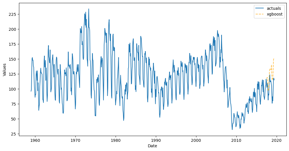
f.plot_test_set();
Score the default Interval
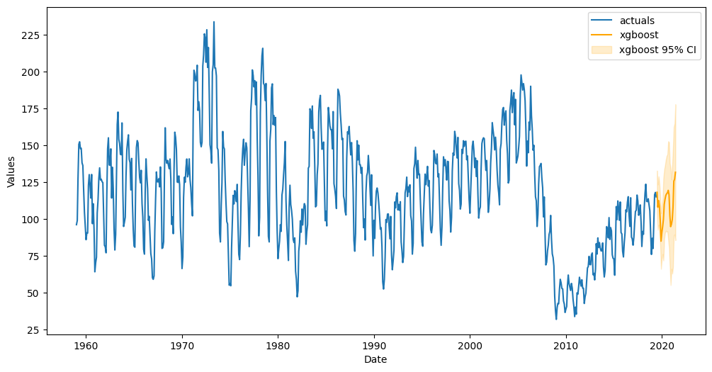
[11]:
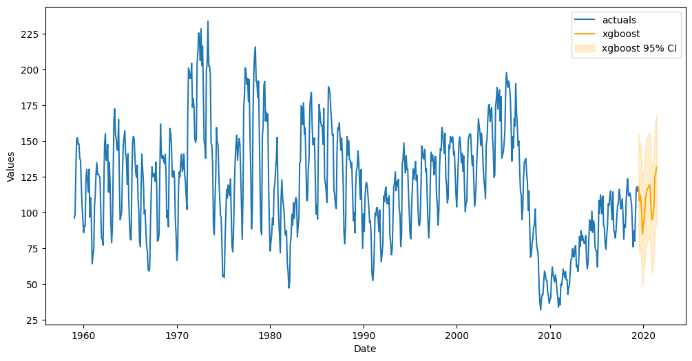
f.plot(ci=True);
[12]:
fig, ax = plt.subplots(figsize=(12,6))
f.plot(ci=True,models='top_1',order_by='TestSetRMSE',ax=ax)
sns.lineplot(
y = 'HOUSTNSA',
x = 'DATE',
data = starts_sep.reset_index(),
ax = ax,
label = 'held-out actuals',
color = 'green',
alpha = 0.7,
)
plt.xlim(pd.Timestamp('2000-01-01'),pd.Timestamp('2021-12-01'))
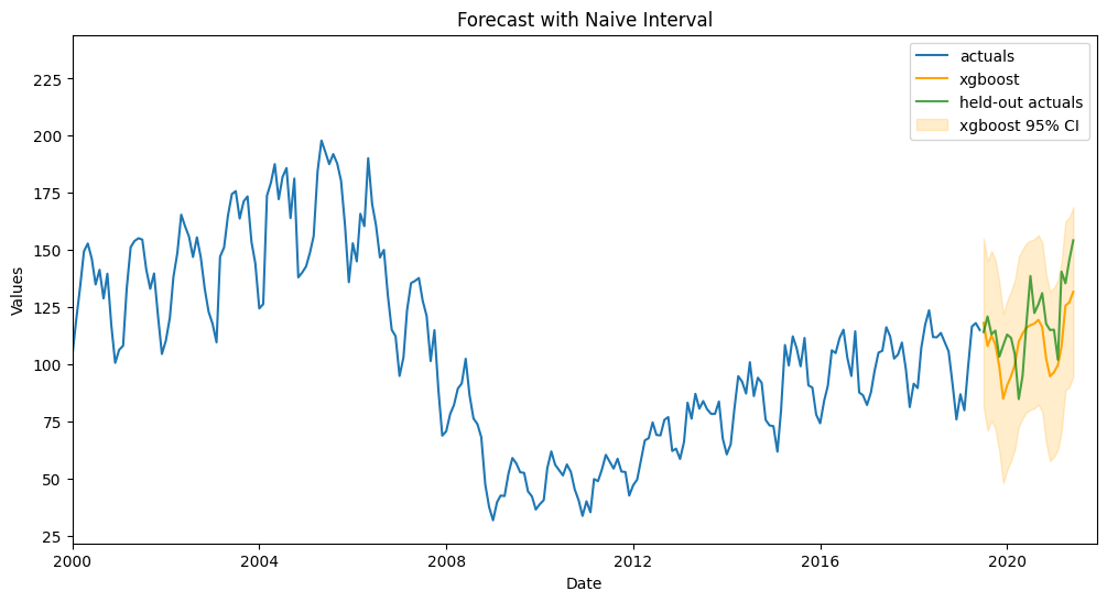
plt.title('Forecast with Naive Interval')
plt.show()
[13]:
print(
    'All confidence intervals for every step'
    ' are {:.2f} units away from the point predictions.'.format(
        f.history['xgboost']['UpperCI'][0] - f.history['xgboost']['Forecast'][0]
    )
)
print(
    'The interval contains {:.2%} of the actual values'.format(
        np.sum(
            [
                1 if a <= uf and a >= lf else 0
                for a, uf, lf in zip(
                    starts_sep,
                    f.history['xgboost']['UpperCI'],
                    f.history['xgboost']['LowerCI']
                )
            ]
        ) / len(starts_sep)
    )
)
All confidence intervals for every step are 37.01 units away from the point predictions.
The interval contains 100.00% of the actual values
Score default interval
[14]:
metrics.msis(
    a = starts_sep,
    uf = f.history['xgboost']['UpperCI'],
    lf = f.history['xgboost']['LowerCI'],
    obs = f.y,
    m = 12,
)
[14]:
4.026554265078705
Step 2: Backtest Pipeline
Iterations need to be at least 20 for 95% intervals.
Length of each prediction in the backtest should match our desired forecast length.
[15]:
%%time
backtest_results = backtest_for_resid_matrix(
    f,
    pipeline=pipeline,
    alpha = .05, # default
    jump_back = 1, # default
)
CPU times: total: 1min 40s
Wall time: 28.5 s
Step 3: Build Residual Matrix
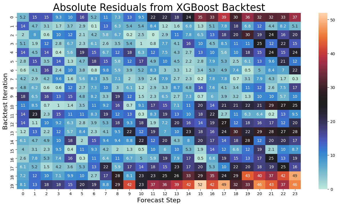
Result is matrix shaped 20x24, each row a backtest iteration, each column a forecast step, each value a residual.
[16]:
backtest_resid_matrix = get_backtest_resid_matrix(backtest_results)
Residual Analytics
[17]:
pd.options.display.max_columns = None
fig, ax = plt.subplots(figsize=(16,8))
mat = pd.DataFrame(np.abs(backtest_resid_matrix[0]['xgboost']))
sns.heatmap(
    mat.round(1),
    annot = True,
    ax = ax,
    cmap = sns.color_palette("icefire", as_cmap=True)
)
plt.ylabel('Backtest Iteration',size=16)
plt.xlabel('Forecast Step',size = 16)
plt.title('Absolute Residuals from XGBoost Backtest',size=25)
plt.show()
[18]:
fig, ax = plt.subplots(1,2,figsize=(16,8))
sns.heatmap(
    pd.DataFrame({'Mean Residuals':mat.mean().round(1)}),
    annot = True,
    cmap = 'cubehelix_r',
    ax = ax[0],
    annot_kws={"fontsize": 16},
)
cbar = ax[0].collections[0].colorbar
cbar.ax.invert_yaxis()
ax[0].set_title('Mean Absolute Residuals',size=20)
ax[0].set_ylabel('Forecast Step',size=15)
ax[0].set_xlabel('')
sns.heatmap(
    pd.DataFrame({'Residuals 95 Percentile':np.percentile(mat, q=95, axis = 0)}),
    annot = True,
    cmap = 'cubehelix_r',
    ax = ax[1],
    annot_kws={"fontsize": 16},
)
cbar = ax[1].collections[0].colorbar
cbar.ax.invert_yaxis()
ax[1].set_title('Absolute Residual 95 Percentiles',size=20)
ax[1].set_ylabel('Forecast Step',size=15)
ax[1].set_xlabel('')
plt.show()
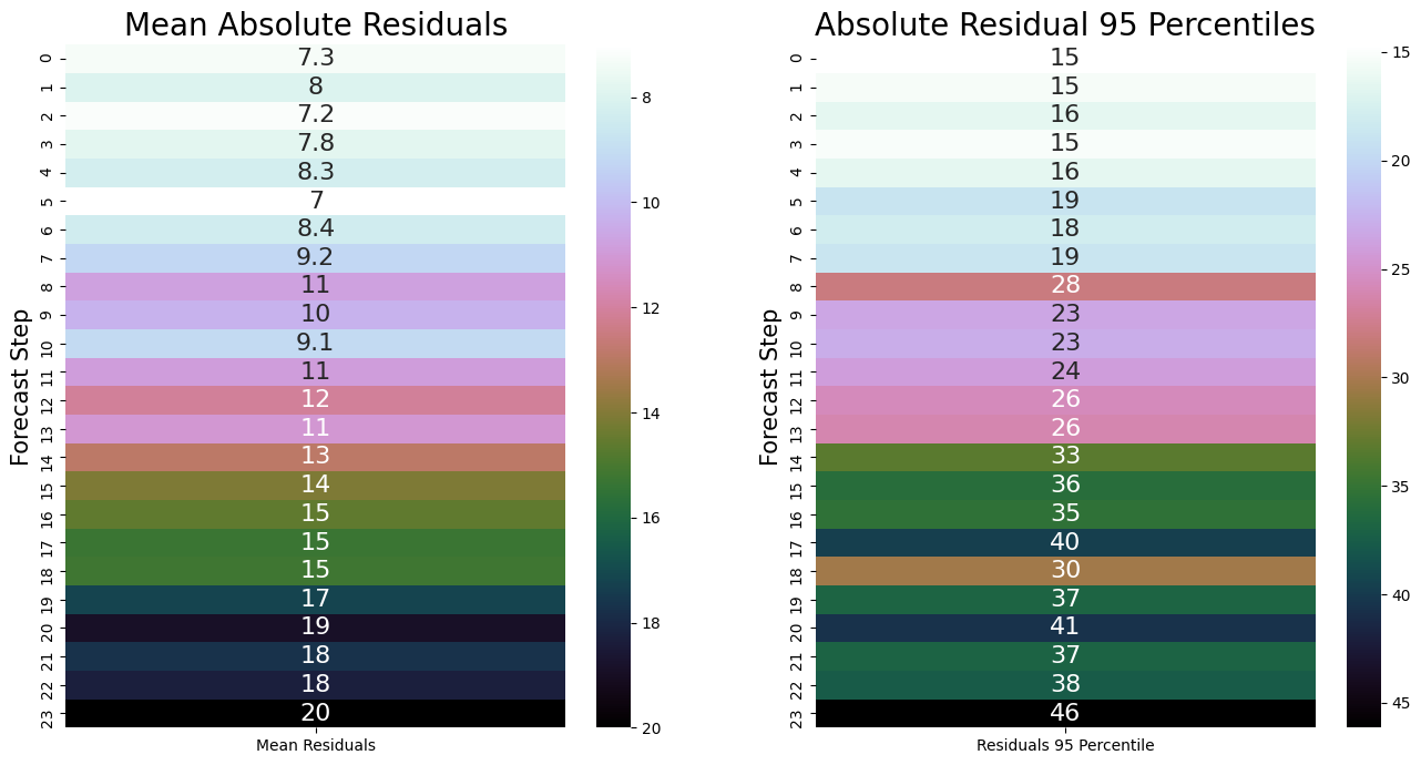
Each step of the forecast will be plus/minus the 95 percentile of the absolute residuals (plot on right).
Step 4: Overwrite Naive Interval with Dynamic Interval
[19]:
overwrite_forecast_intervals(f,backtest_resid_matrix=backtest_resid_matrix)
[20]:
f.plot(ci=True);
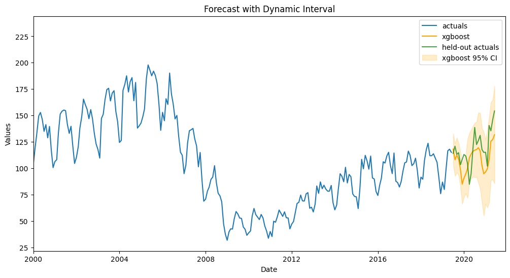
[21]:
fig, ax = plt.subplots(figsize=(12,6))
f.plot(ci=True,models='top_1',order_by='TestSetRMSE',ax=ax)
sns.lineplot(
    y = 'HOUSTNSA',
    x = 'DATE',
    data = starts_sep.reset_index(),
    ax = ax,
    label = 'held-out actuals',
    color = 'green',
    alpha = 0.7,
)
plt.xlim(pd.Timestamp('2000-01-01'),pd.Timestamp('2021-12-01'))
plt.title('Forecast with Dynamic Interval')
plt.show()
Score dynamic interval
[22]:
metrics.msis(
    a = starts_sep,
    uf = f.history['xgboost']['UpperCI'],
    lf = f.history['xgboost']['LowerCI'],
    obs = f.y,
    m = 12,
)
[22]:
3.919628517087574
It is a small improvement, but still an improvement!
[23]:
print(
    'The intervals are on average {:.2f} units away from the point predictions.'.format(
        np.mean(np.percentile(mat, q=95, axis = 0))
    )

)
print(
    'The interval contains {:.2%} of the actual values'.format(
        np.sum(
            [
                1 if a <= uf and a >= lf else 0
                for a, uf, lf in zip(
                    starts_sep,
                    f.history['xgboost']['UpperCI'],
                    f.history['xgboost']['LowerCI']
                )
            ]
        ) / len(starts_sep)
    )
)
The intervals are on average 27.36 units away from the point predictions.
The interval contains 87.50% of the actual values
Other Backtest Uses
We can also use the backtest results to report average error metrics over 20 out-of-sample sets.
[24]:
backtest_metrics(backtest_results,mets=['rmse','mae','bias'])[['Average']]
[24]:
| Average | ||
|---|---|---|
| Model | Metric | |
| xgboost | rmse | 14.083597 |
| mae | 12.144780 | |
| bias | 239.430706 |
[25]:
# actual rmse on out-of-sample data
metrics.rmse(starts_sep,f.history['xgboost']['Forecast'])
[25]:
16.208569138706174
[ ]: