Multivariate Forecasting

This notebook outlines an example of scalecast using multiple series to forecast one another using scikit-learn models.

The data is available on Kaggle: https://www.kaggle.com/datasets/neuromusic/avocado-prices

See the blog post: https://towardsdatascience.com/multiple-series-forecast-them-together-with-any-sklearn-model-96319d46269

[1]:

import pandas as pd
import numpy as np
import seaborn as sns
import matplotlib
import matplotlib.ticker as ticker
import matplotlib.pyplot as plt
from scalecast.Forecaster import Forecaster
from scalecast.MVForecaster import MVForecaster
from scalecast.multiseries import export_model_summaries
from scalecast import GridGenerator

[2]:

# read data
data = pd.read_csv('avocado.csv',parse_dates=['Date']).sort_values(['Date'])
# sort appropriately (not doing this could cause issues)
data = data.sort_values(['region','type','Date'])

We will be forecasting the organic and conventional avocado sales from California only.

[3]:

data_cali = data.loc[data['region'] == 'California']
data_cali_org = data_cali.loc[data_cali['type'] == 'organic']
data_cali_con = data_cali.loc[data_cali['type'] == 'conventional']

Choose Models and Import Validation Grids

[4]:

# download template validation grids (will not overwrite existing Grids.py file by default)
models = ('mlr','elasticnet','knn','rf','gbt','xgboost','mlp')
GridGenerator.get_example_grids()
GridGenerator.get_mv_grids()

EDA

Plot

[5]:

fig, ax = plt.subplots(figsize=(12,6))
sns.lineplot(
    x='Date',
    y='Total Volume',
    data=data_cali_con,
    label='conventional',
    ax=ax,
    color='black',
    legend=False
)
plt.ylabel('Conventional',size=16)
ax2 = ax.twinx()
sns.lineplot(
    x='Date',
    y='Total Volume',
    data=data_cali_org,
    label='organic',
    ax=ax2,
    color='#B2C248',
    legend=False
)
ax.figure.legend()
plt.ylabel('Organic',size=16)
ax.yaxis.set_major_formatter(ticker.StrMethodFormatter('{x:,.0f}'))
ax2.yaxis.set_major_formatter(ticker.StrMethodFormatter('{x:,.0f}'))
plt.suptitle('Conventional and Organic Avocado Sale Volumes',size=20)
plt.show()

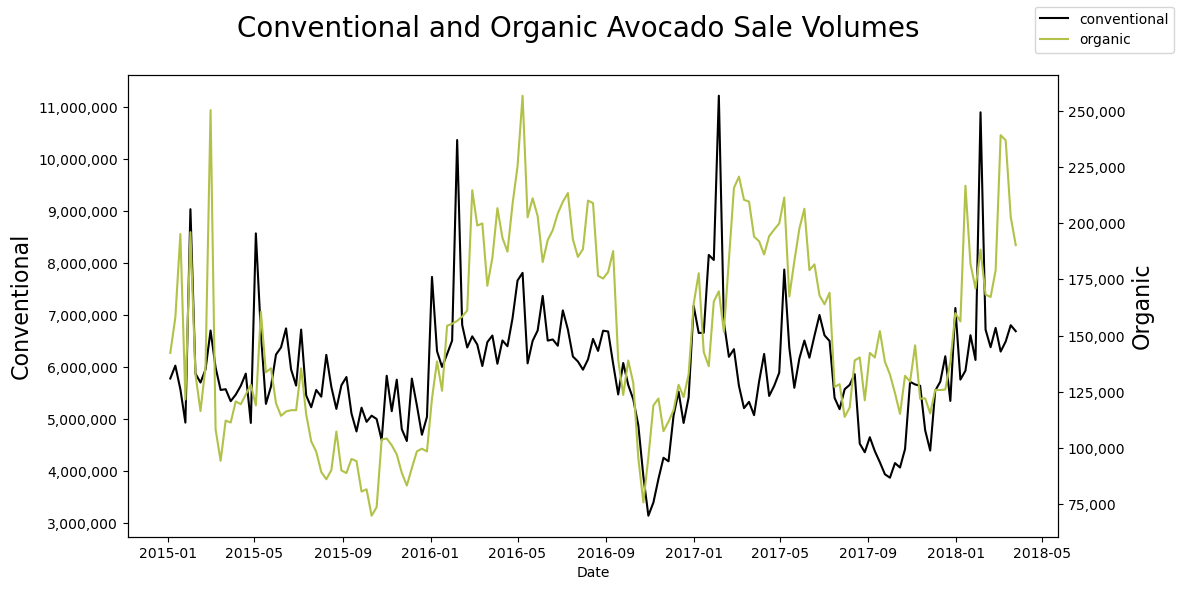
../_images/multivariate_multivariate_9_0.png

Examine Correlation between the series

[6]:

corr = np.corrcoef(data_cali_org['Total Volume'].values,data_cali_con['Total Volume'].values)[0,1]
print('{:.2%}'.format(corr))

48.02%

Load into Forecaster from scalecast

[7]:

fcon = Forecaster(
    y=data_cali_con['Total Volume'],
    current_dates = data_cali_con['Date'],
    test_length = .2,
    future_dates = 52,
    validation_length = 4,
    metrics = ['rmse','r2'],
    cis = True,
)
fcon

[7]:

Forecaster(
    DateStartActuals=2015-01-04T00:00:00.000000000
    DateEndActuals=2018-03-25T00:00:00.000000000
    Freq=W-SUN
    N_actuals=169
    ForecastLength=52
    Xvars=[]
    TestLength=33
    ValidationMetric=rmse
    ForecastsEvaluated=[]
    CILevel=0.95
    CurrentEstimator=mlr
    GridsFile=Grids
)

[8]:

forg = Forecaster(
    y=data_cali_org['Total Volume'],
    current_dates = data_cali_org['Date'],
    test_length = .2,
    future_dates = 52,
    validation_length = 4,
    metrics = ['rmse','r2'],
    cis = True,
)
forg

[8]:

Forecaster(
    DateStartActuals=2015-01-04T00:00:00.000000000
    DateEndActuals=2018-03-25T00:00:00.000000000
    Freq=W-SUN
    N_actuals=169
    ForecastLength=52
    Xvars=[]
    TestLength=33
    ValidationMetric=rmse
    ForecastsEvaluated=[]
    CILevel=0.95
    CurrentEstimator=mlr
    GridsFile=Grids
)

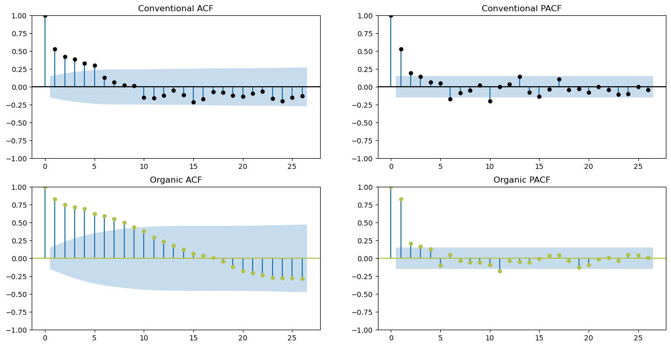
ACF and PACF Plots

[9]:

figs, axs = plt.subplots(2, 2,figsize=(16,8))
fcon.plot_acf(
    ax=axs[0,0],
    title='Conventional ACF',
    lags=26,
    color='black'
)
fcon.plot_pacf(
    ax=axs[0,1],
    title='Conventional PACF',
    lags=26,
    color='black',
    method='ywm'
)
forg.plot_acf(
    ax=axs[1,0],
    title='Organic ACF',
    lags=26,
    color='#B2C248'
)
forg.plot_pacf(
    ax=axs[1,1],
    title='Organic PACF',
    lags=26,
    color='#B2C248',
    method='ywm'
)
plt.show()

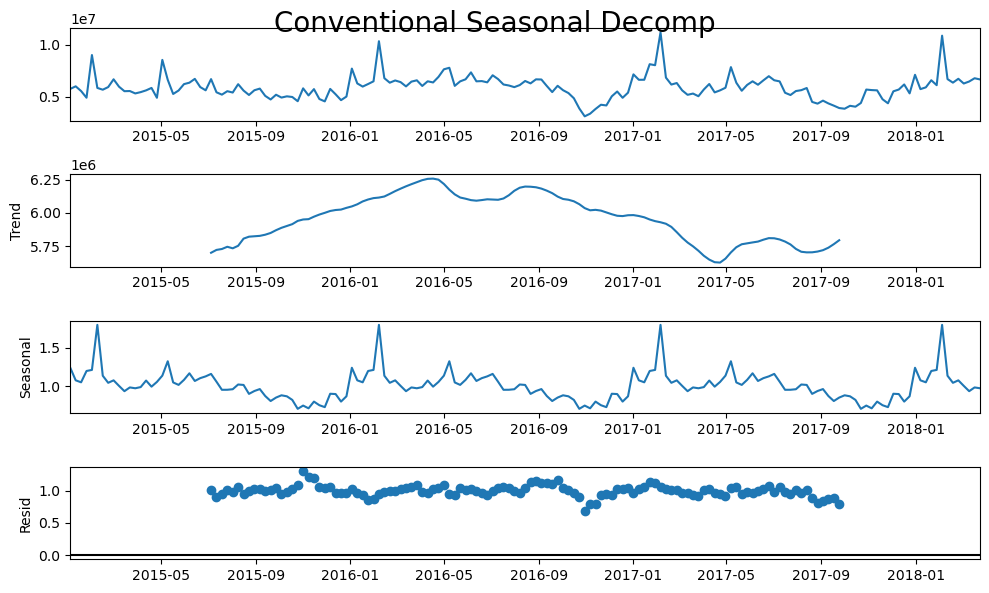
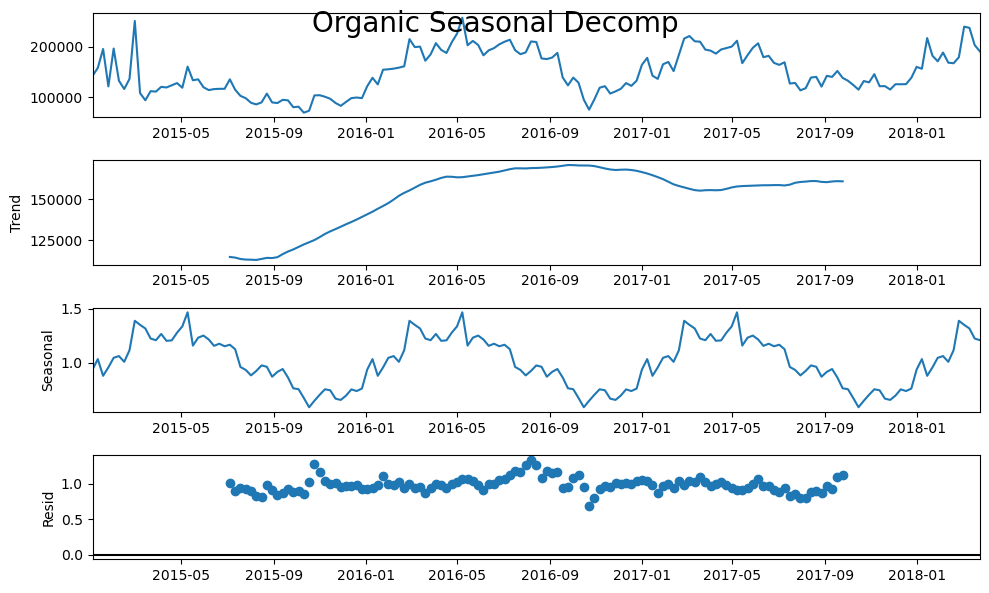
../_images/multivariate_multivariate_16_0.png

Seasonal Decomposition Plots

[10]:

plt.rc("figure",figsize=(10,6))
fcon.seasonal_decompose(model='mul').plot()
plt.suptitle('Conventional Seasonal Decomp',size=20)
plt.show()

../_images/multivariate_multivariate_18_0.png

[11]:

forg.seasonal_decompose(model='mul').plot()
plt.suptitle('Organic Seasonal Decomp',size=20)
plt.show()

../_images/multivariate_multivariate_19_0.png

Check Stationarity

[12]:

critical_pval = 0.05
print('-'*100)
print('Conventional Augmented Dickey-Fuller results:')
stat, pval, _, _, _, _ = fcon.adf_test(full_res=True)
print('the test-stat value is: {:.2f}'.format(stat))
print('the p-value is {:.4f}'.format(pval))
print('the series is {}'.format('stationary' if pval < critical_pval else 'not stationary'))
print('-'*100)
print('Organic Augmented Dickey-Fuller results:')
stat, pval, _, _, _, _ = forg.adf_test(full_res=True)
print('the test-stat value is: {:.2f}'.format(stat))
print('the p-value is {:.4f}'.format(pval))
print('the series is {}'.format('stationary' if pval < critical_pval else 'not stationary'))
print('-'*100)

----------------------------------------------------------------------------------------------------
Conventional Augmented Dickey-Fuller results:
the test-stat value is: -3.35
the p-value is 0.0128
the series is stationary
----------------------------------------------------------------------------------------------------
Organic Augmented Dickey-Fuller results:
the test-stat value is: -2.94
the p-value is 0.0404
the series is stationary
----------------------------------------------------------------------------------------------------

Scalecast - Univariate

Load Objects with Xvars:

Find best combination of trend, lags, and seasonality monitoring the validation set (4 observations before the test set)

[13]:

for f in (fcon,forg):
    f.auto_Xvar_select(
        estimator = 'elasticnet',
        monitor = 'ValidationMetricValue',
        irr_cycles = [26], # try irregular semi-annual seaosnality
        cross_validate=True,
        cvkwargs={
            'k':3,
            'test_length':13,
            'space_between_sets':4,
        }
    )
    print(f)

Forecaster(
    DateStartActuals=2015-01-04T00:00:00.000000000
    DateEndActuals=2018-03-25T00:00:00.000000000
    Freq=W-SUN
    N_actuals=169
    ForecastLength=52
    Xvars=['weeksin', 'weekcos', 'monthsin', 'monthcos', 'quartersin', 'quartercos', 'AR1', 'AR2', 'AR3', 'AR4', 'AR5', 'AR6', 'AR7', 'AR8', 'AR9', 'AR10', 'AR11', 'AR12', 'AR13', 'AR14', 'AR15', 'AR16', 'AR17', 'AR18', 'AR19', 'AR20', 'AR21', 'AR22', 'AR23', 'AR24', 'AR25', 'AR26', 'AR27', 'AR28', 'AR29', 'AR30', 'AR31', 'AR32', 'AR33']
    TestLength=33
    ValidationMetric=rmse
    ForecastsEvaluated=[]
    CILevel=0.95
    CurrentEstimator=mlr
    GridsFile=Grids
)
Forecaster(
    DateStartActuals=2015-01-04T00:00:00.000000000
    DateEndActuals=2018-03-25T00:00:00.000000000
    Freq=W-SUN
    N_actuals=169
    ForecastLength=52
    Xvars=['lnt', 'AR1', 'AR2', 'AR3', 'AR4', 'AR5', 'AR6', 'AR7', 'AR8', 'AR9', 'AR10', 'AR11', 'AR12', 'AR13', 'AR14', 'AR15', 'AR16', 'AR17', 'AR18', 'AR19', 'AR20', 'AR21', 'AR22', 'AR23', 'AR24', 'AR25', 'AR26', 'AR27', 'AR28', 'AR29', 'AR30', 'AR31', 'AR32', 'AR33']
    TestLength=33
    ValidationMetric=rmse
    ForecastsEvaluated=[]
    CILevel=0.95
    CurrentEstimator=mlr
    GridsFile=Grids
)

Tune and Forecast with Selected Models

Find optimal hyperparameters using the four out-of-sample observations then test results on test set

Conventional

[14]:

fcon.tune_test_forecast(models,feature_importance=True)
best_model_con_uni = fcon.order_fcsts()[0]
fcon.set_estimator('combo')
fcon.manual_forecast(how='weighted')

2023-04-11 15:32:19.815928: I tensorflow/core/platform/cpu_feature_guard.cc:193] This TensorFlow binary is optimized with oneAPI Deep Neural Network Library (oneDNN) to use the following CPU instructions in performance-critical operations:  SSE4.1 SSE4.2
To enable them in other operations, rebuild TensorFlow with the appropriate compiler flags.

[15]:

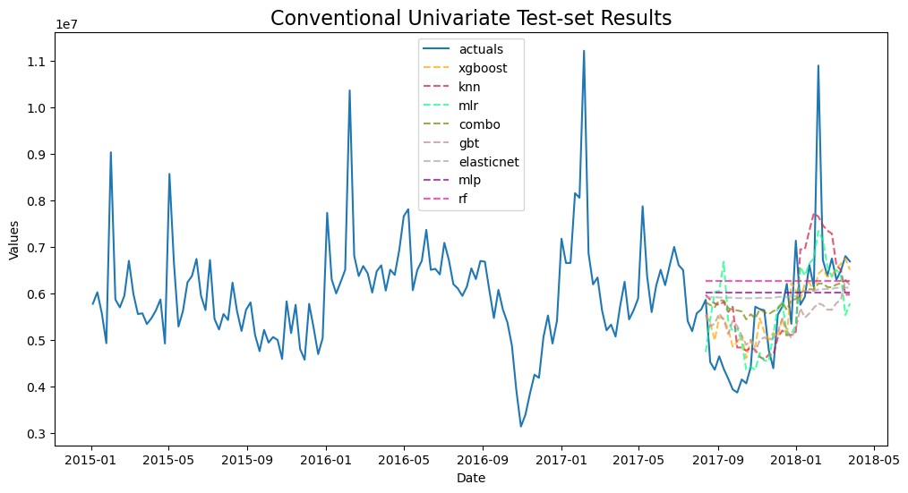
fcon.plot_test_set(order_by='TestSetRMSE')
plt.title('Conventional Univariate Test-set Results',size=16)
plt.show()

../_images/multivariate_multivariate_26_0.png

Organic

[16]:

forg.tune_test_forecast(models,feature_importance=True)
best_model_org_uni = forg.order_fcsts()[0]
forg.set_estimator('combo')
forg.manual_forecast(how='weighted')

[17]:

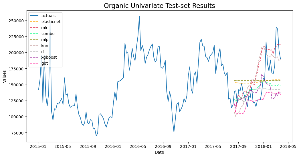
forg.plot_test_set(order_by='TestSetRMSE')
plt.title('Organic Univariate Test-set Results',size=16)
plt.show()

../_images/multivariate_multivariate_29_0.png

Model Summaries

[22]:

pd.set_option('display.float_format',  '{:.4f}'.format)
ms = export_model_summaries({'Conventional':fcon,'Organic':forg},determine_best_by='TestSetRMSE')
ms[
    [
        'ModelNickname',
        'Series',
        'TestSetRMSE',
        'TestSetR2',
        'InSampleRMSE',
        'InSampleR2',
        'best_model'
    ]
]

[22]:

	ModelNickname	Series	TestSetRMSE	TestSetR2	InSampleRMSE	InSampleR2	best_model
0	xgboost	Conventional	1006995.5599	0.4446	3.6627	1.0000	True
1	knn	Conventional	1131608.0344	0.2987	817774.1332	0.5510	False
2	mlr	Conventional	1149633.3896	0.2761	758866.6492	0.6133	False
3	combo	Conventional	1212096.9382	0.1953	688989.9601	0.6813	False
4	gbt	Conventional	1220551.0383	0.1841	194073.1900	0.9747	False
5	elasticnet	Conventional	1337617.6356	0.0201	1143622.0298	0.1218	False
6	mlp	Conventional	1405812.4388	-0.0824	1220380.8148	-0.0000	False
7	rf	Conventional	1491918.2868	-0.2191	1223366.9295	-0.0049	False
8	elasticnet	Organic	31734.3993	0.1053	37019.4163	0.2451	True
9	mlr	Organic	31826.3068	0.1001	15369.3197	0.8699	False
10	combo	Organic	32193.1479	0.0793	13693.4548	0.8967	False
11	mlp	Organic	33604.8672	-0.0032	42607.8305	-0.0000	False
12	knn	Organic	35461.8762	-0.1172	13801.7064	0.8951	False
13	rf	Organic	35785.6551	-0.1377	9688.4987	0.9483	False
14	xgboost	Organic	37617.5747	-0.2571	0.6991	1.0000	False
15	gbt	Organic	40632.6313	-0.4667	7511.2968	0.9689	False

Because running so many models can cause overfitting on the test set, we can check the average test error between all models to get another metric of how effective our modeling process is.

[23]:

print('-'*100)
for series in ms['Series'].unique():
    print('univariate average test MAPE for {}: {:.4f}'.format(series,ms.loc[ms['Series'] == series,'TestSetRMSE'].mean()))
    print('univariate average test R2 for {}: {:.2f}'.format(series,ms.loc[ms['Series'] == series,'TestSetR2'].mean()))
    print('-'*100)

----------------------------------------------------------------------------------------------------
univariate average test MAPE for Conventional: 1244529.1652
univariate average test R2 for Conventional: 0.14
----------------------------------------------------------------------------------------------------
univariate average test MAPE for Organic: 34857.0573
univariate average test R2 for Organic: -0.09
----------------------------------------------------------------------------------------------------

These are interesting error metrics, but a lot of models, including XGBoost and GBT appear to be overfitting. Let’s see if we can beat the results with a multivariate approach.

Scalecast - Multivariate

Set MV Parameters

Forecast horizon already set
Xvars already set
Test size must be set: 20%
Validation size must be set: 4 periods

[24]:

mvf = MVForecaster(
    fcon,forg,
    names=['Conventional','Organic'],
    test_length = .2,
    valiation_length = 4,
    cis = True,
    metrics = ['rmse','r2'],
) # init the mvf object
mvf

[24]:

MVForecaster(
    DateStartActuals=2015-01-04T00:00:00.000000000
    DateEndActuals=2018-03-25T00:00:00.000000000
    Freq=W-SUN
    N_actuals=169
    N_series=2
    SeriesNames=['Conventional', 'Organic']
    ForecastLength=52
    Xvars=['weeksin', 'weekcos', 'monthsin', 'monthcos', 'quartersin', 'quartercos', 'lnt']
    TestLength=33
    ValidationLength=1
    ValidationMetric=rmse
    ForecastsEvaluated=[]
    CILevel=0.95
    CurrentEstimator=mlr
    OptimizeOn=mean
    GridsFile=MVGrids
)

The lags from each Forecaster object dropped but they will be added into the multivariate models differently.

View Series Correlation

[25]:

mvf.corr()

[25]:

	Conventional	Organic
Conventional	1.0000	0.4802
Organic	0.4802	1.0000

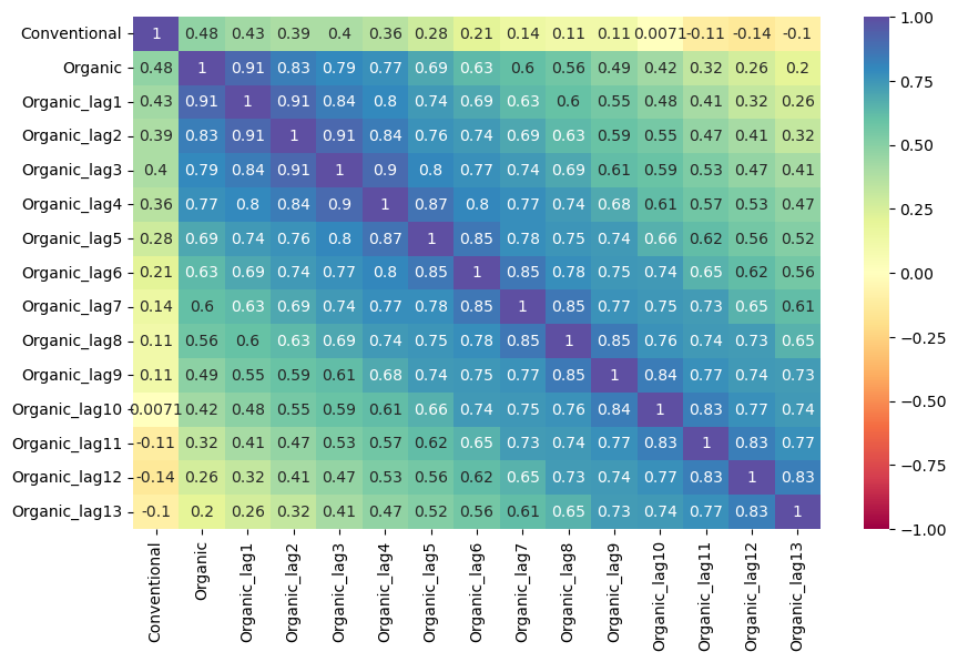
View Series Correlation with each others’ lags

[26]:

mvf.corr_lags(
    y='Conventional',
    x='Organic',
    lags=13,
    disp='heatmap',
    annot=True,
    vmin=-1,
    vmax=1,
    cmap = 'Spectral',
)
plt.show()

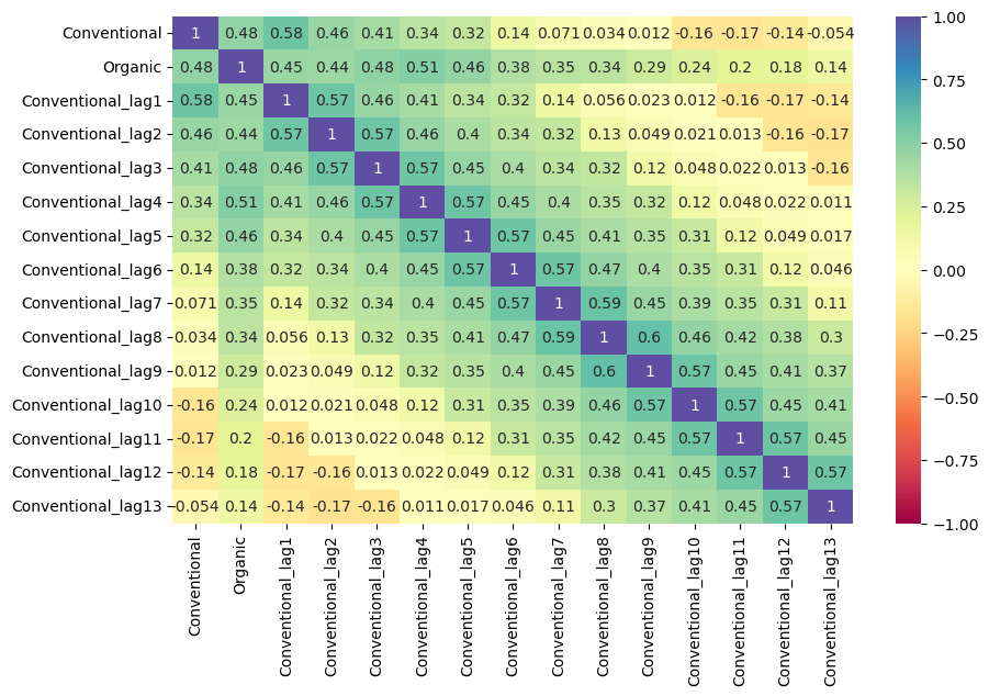
../_images/multivariate_multivariate_41_0.png

[27]:

mvf.corr_lags(
    y='Organic',
    x='Conventional',
    lags=13,
    disp='heatmap',
    annot=True,
    vmin=-1,
    vmax=1,
    cmap = 'Spectral',
)
plt.show()

../_images/multivariate_multivariate_42_0.png

Set Optimize On

If predicting one series is more important than predicting the other, you can use this code to let the code know to favor one over the other
By default, it uses the mean error metrics between all series

[28]:

# how to optimize on one series
mvf.set_optimize_on('Organic')
# how to optimize using a weighted avarage
mvf.add_optimizer_func(lambda x: x[0]*.25 + x[1]*.75,'weighted')
mvf.set_optimize_on('weighted')
# how to optimize on the average of both/all series (default)
mvf.set_optimize_on('mean')

Tune and Test with Selected Models

[29]:

mvf.tune_test_forecast(models)
mvf.set_best_model(determine_best_by='TestSetRMSE')

[30]:

# not plotting both series at the same time because they have significantly different scales
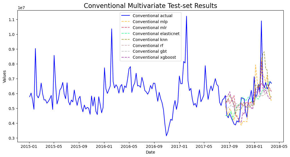
mvf.plot_test_set(series='Conventional',put_best_on_top=True)
plt.title('Conventional Multivariate Test-set Results',size=16)
plt.show()

../_images/multivariate_multivariate_47_0.png

[31]:

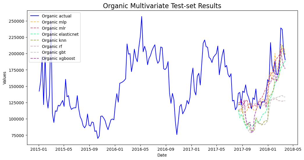
mvf.plot_test_set(series='Organic',put_best_on_top=True)
plt.title('Organic Multivariate Test-set Results',size=16)
plt.show()

../_images/multivariate_multivariate_48_0.png

Export Model Summaries

[32]:

pd.options.display.max_colwidth = 100
results = mvf.export('model_summaries')
results[
    [
        'ModelNickname',
        'Series',
        'HyperParams',
        'TestSetRMSE',
        'TestSetR2',
        'InSampleRMSE',
        'InSampleR2',
        'Lags'
    ]
]

[32]:

	ModelNickname	Series	HyperParams	TestSetRMSE	TestSetR2	InSampleRMSE	InSampleR2	Lags
0	mlp	Conventional	{'activation': 'relu', 'hidden_layer_sizes': (25, 25), 'solver': 'lbfgs', 'normalizer': 'minmax'...	976640.7441	0.4776	726613.9497	0.6134	3
1	mlr	Conventional	{'normalizer': None}	1090383.4159	0.3488	889221.9216	0.4209	3
2	elasticnet	Conventional	{'alpha': 0.9, 'l1_ratio': 0.75, 'normalizer': None}	1053128.2384	0.3926	752345.3345	0.5889	13
3	knn	Conventional	{'n_neighbors': 4, 'weights': 'uniform'}	1178477.0280	0.2394	663362.5001	0.6804	13
4	rf	Conventional	{'max_depth': 5, 'n_estimators': 100}	1202344.6297	0.2082	343671.0745	0.9142	13
5	gbt	Conventional	{'max_depth': 2, 'max_features': None}	1124594.8764	0.3073	259436.1165	0.9511	13
6	xgboost	Conventional	{'max_depth': 2}	974696.0984	0.4797	233374.4324	0.9597	1
7	mlp	Organic	{'activation': 'relu', 'hidden_layer_sizes': (25, 25), 'solver': 'lbfgs', 'normalizer': 'minmax'...	20920.8153	0.6112	16252.8787	0.8544	3
8	mlr	Organic	{'normalizer': None}	17923.9250	0.7146	20380.0266	0.7710	3
9	elasticnet	Organic	{'alpha': 0.9, 'l1_ratio': 0.75, 'normalizer': None}	37629.9902	-0.2580	14968.7668	0.8746	13
10	knn	Organic	{'n_neighbors': 4, 'weights': 'uniform'}	36796.6649	-0.2029	12551.0264	0.9118	13
11	rf	Organic	{'max_depth': 5, 'n_estimators': 100}	43547.8368	-0.6848	8941.5674	0.9552	13
12	gbt	Organic	{'max_depth': 2, 'max_features': None}	50265.9563	-1.2447	7325.5184	0.9700	13
13	xgboost	Organic	{'max_depth': 2}	26986.2883	0.3530	6488.8763	0.9767	1

Import a Foreign Sklearn Estimator for Ensemble Modeling

[33]:

from sklearn.ensemble import StackingRegressor
from sklearn.linear_model import LinearRegression
from sklearn.linear_model import ElasticNet
from sklearn.neural_network import MLPRegressor
from sklearn.neighbors import KNeighborsRegressor
from xgboost import XGBRegressor
estimators = [
    (
        'mlr',
        LinearRegression()
    ),
    (
        'elasticnet',
        ElasticNet(
            **{
                k:v for k,v in (
                    results.loc[
                        results['ModelNickname'] == 'elasticnet',
                        'HyperParams',
                    ].values[0]
                ).items() if k != 'normalizer'
              }
        )
    ),
    (
        'mlp',
        MLPRegressor(
            **{
                k:v for k,v in (
                    results.loc[
                        results['ModelNickname'] == 'mlp',
                        'HyperParams',
                    ].values[0]
                ).items() if k != 'normalizer'
              }
        )
    )
]

final_estimator = KNeighborsRegressor(
    **{
        k:v for k,v in (
            results.loc[
                results['ModelNickname'] == 'knn',
                'HyperParams',
            ].values[0]
        ).items() if k != 'normalizer'
      }
)

[34]:

mvf.add_sklearn_estimator(StackingRegressor,'stacking')
mvf.set_estimator('stacking')
mvf.manual_forecast(estimators=estimators,final_estimator=final_estimator,lags=13)

[35]:

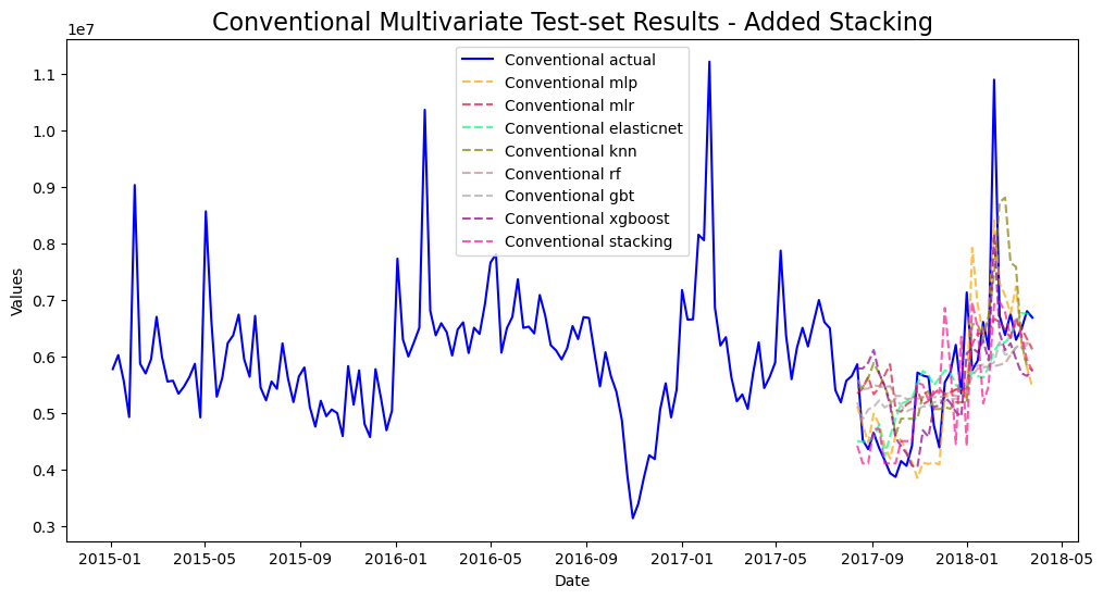
mvf.plot_test_set(series='Conventional',put_best_on_top=True)
plt.title('Conventional Multivariate Test-set Results - Added Stacking',size=16)
plt.show()

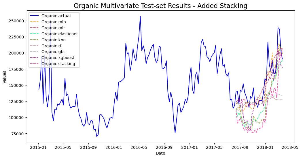
../_images/multivariate_multivariate_54_0.png

[36]:

mvf.plot_test_set(series='Organic',put_best_on_top=True)
plt.title('Organic Multivariate Test-set Results - Added Stacking',size=16)
plt.show()

../_images/multivariate_multivariate_55_0.png

[37]:

mvf.set_best_model(determine_best_by='TestSetRMSE')
results2 = mvf.export('model_summaries')
results2 = results2[
    [
        'ModelNickname',
        'Series',
        'TestSetRMSE',
        'TestSetR2',
        'InSampleRMSE',
        'InSampleR2',
        'Lags',
        'best_model'
    ]
]

results2

[37]:

	ModelNickname	Series	TestSetRMSE	TestSetR2	InSampleRMSE	InSampleR2	Lags	best_model
0	mlp	Conventional	976640.7441	0.4776	726613.9497	0.6134	3	True
1	mlr	Conventional	1090383.4159	0.3488	889221.9216	0.4209	3	False
2	elasticnet	Conventional	1053128.2384	0.3926	752345.3345	0.5889	13	False
3	knn	Conventional	1178477.0280	0.2394	663362.5001	0.6804	13	False
4	rf	Conventional	1202344.6297	0.2082	343671.0745	0.9142	13	False
5	gbt	Conventional	1124594.8764	0.3073	259436.1165	0.9511	13	False
6	xgboost	Conventional	974696.0984	0.4797	233374.4324	0.9597	1	False
7	stacking	Conventional	1098442.4396	0.3392	838807.3770	0.4890	13	False
8	mlp	Organic	20920.8153	0.6112	16252.8787	0.8544	3	True
9	mlr	Organic	17923.9250	0.7146	20380.0266	0.7710	3	False
10	elasticnet	Organic	37629.9902	-0.2580	14968.7668	0.8746	13	False
11	knn	Organic	36796.6649	-0.2029	12551.0264	0.9118	13	False
12	rf	Organic	43547.8368	-0.6848	8941.5674	0.9552	13	False
13	gbt	Organic	50265.9563	-1.2447	7325.5184	0.9700	13	False
14	xgboost	Organic	26986.2883	0.3530	6488.8763	0.9767	1	False
15	stacking	Organic	47928.2496	-1.0407	17511.0377	0.8284	13	False

[38]:

print('-'*100)
for series in results2['Series'].unique():
    print('multivariate average test MAPE for {}: {:.4f}'.format(series,results2.loc[results2['Series'] == series,'TestSetRMSE'].mean()))
    print('multivariate average test R2 for {}: {:.2f}'.format(series,results2.loc[results2['Series'] == series,'TestSetR2'].mean()))
    print('-'*100)

----------------------------------------------------------------------------------------------------
multivariate average test MAPE for Conventional: 1087338.4338
multivariate average test R2 for Conventional: 0.35
----------------------------------------------------------------------------------------------------
multivariate average test MAPE for Organic: 35249.9658
multivariate average test R2 for Organic: -0.22
----------------------------------------------------------------------------------------------------

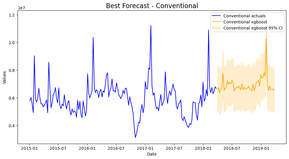
Plot Final Forecasts

[39]:

best_model_con = (
    results2.loc[results2['Series'] == 'Conventional']
    .sort_values('TestSetR2',ascending=False)
    .iloc[0,0]
)

[40]:

mvf.plot(series='Conventional',models=best_model_con,ci=True)
plt.title('Best Forecast - Conventional',size=16)
plt.show()

../_images/multivariate_multivariate_60_0.png

[41]:

best_model_org = (
    results2.loc[results2['Series'] == 'Organic']
    .sort_values('TestSetR2',ascending=False)
    .iloc[0,0]
)

[42]:

mvf.plot(series='Organic',models=best_model_org,ci=True)
plt.title('Best Forecast - Organic',size=16)
plt.show()

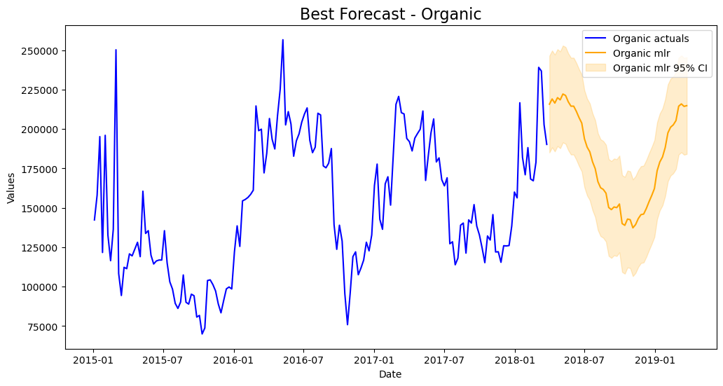
../_images/multivariate_multivariate_62_0.png

All-in-all, better results on the test-set were obtained by using the multivariate approach.

Multivariate Backtest

Just like in univariate modeling, we can evaluate the results of this modeling approach using backtesting.

[46]:

from scalecast.Pipeline import Transformer, Reverter, MVPipeline
from scalecast.util import backtest_metrics

def mvforecaster(mvf):
    mvf.add_seasonal_regressors('month','quarter',raw=False,sincos=True)
    mvf.tune_test_forecast(
        models=[best_model_con,best_model_org],
    )

pipeline = MVPipeline(
    steps = [('Forecast',mvforecaster)],
    validation_length = 4,
)

[47]:

backtest_results = pipeline.backtest(
    fcon,
    forg,
    cis=False,
    test_length = 0,
    fcst_length = 52,
    jump_back = 4,
    n_iter = 3,
)

[48]:

backtest_metrics(
    backtest_results,
    mets=['rmse','r2'],
    names=['Conventional','Organic'],
)

[48]:

			Iter0	Iter1	Iter2	Average
Series	Model	Metric
Conventional	xgboost	rmse	1147549.7983	1406113.2605	1291947.8525	1281870.3037
	xgboost	r2	0.0323	-0.4901	-0.2085	-0.2221
	mlr	rmse	1182695.7635	1091062.5392	1004623.8802	1092794.0610
	mlr	r2	-0.0278	0.1028	0.2693	0.1148
Organic	xgboost	rmse	38107.4049	48419.8474	50356.9359	45628.0627
	xgboost	r2	-0.3062	-1.3092	-1.3834	-0.9996
	mlr	rmse	34053.1727	29246.3029	21894.3284	28397.9347
	mlr	r2	-0.0430	0.1575	0.5495	0.2213

[ ]: