Meta Prophet

Prophet is a procedure for forecasting time series data based on an additive model where non-linear trends are fit with yearly, weekly, and daily seasonality, plus holiday effects. It works best with time series that have strong seasonal effects and several seasons of historical data. Prophet is robust to missing data and shifts in the trend, and typically handles outliers well.It is designed to se automatically find a good set of hyperparameters for the model in an effort to make forrecast for time series with seasonality and trends.

The Prophet model is not autoregressive, like ARIMA, exponential smoothing, and the other methods we study in a typical time series course (including my own).

The 3 components are:

1. The trend g(t) which can be either linear or logistic.

2. The seasonality s(t), modeled using a Fourier series.

3. The holiday component h(t), which is essentially a one-hot vector “dotted” with a vector of weights, each representing the contribution from their respective holiday.

In this notebook, following concepts are covered:

- Loading time-series

- EDA

- Preparing the data for modeling

- Implementing prophet model

- Evaluating the results

Data: https://www.kaggle.com/datasets/bobnau/daily-website-visitors

Install prophet: pip install prophet

Special thanks to Zohoor Nezhad Halafi for contributing this notebook! Connect with her on LinkedIn.

import pandas as pd
import numpy as np
import seaborn as sns
import matplotlib.pyplot as plt
from scalecast.Forecaster import Forecaster

sns.set(rc={'figure.figsize':(16,8)})

Loading time series

data = pd.read_csv('daily-website-visitors.csv',parse_dates=['Date'])

data=data[['First.Time.Visits','Date']]

data.head()

	First.Time.Visits	Date
0	1430	2014-09-14
1	2297	2014-09-15
2	2352	2014-09-16
3	2327	2014-09-17
4	2130	2014-09-18

EDA

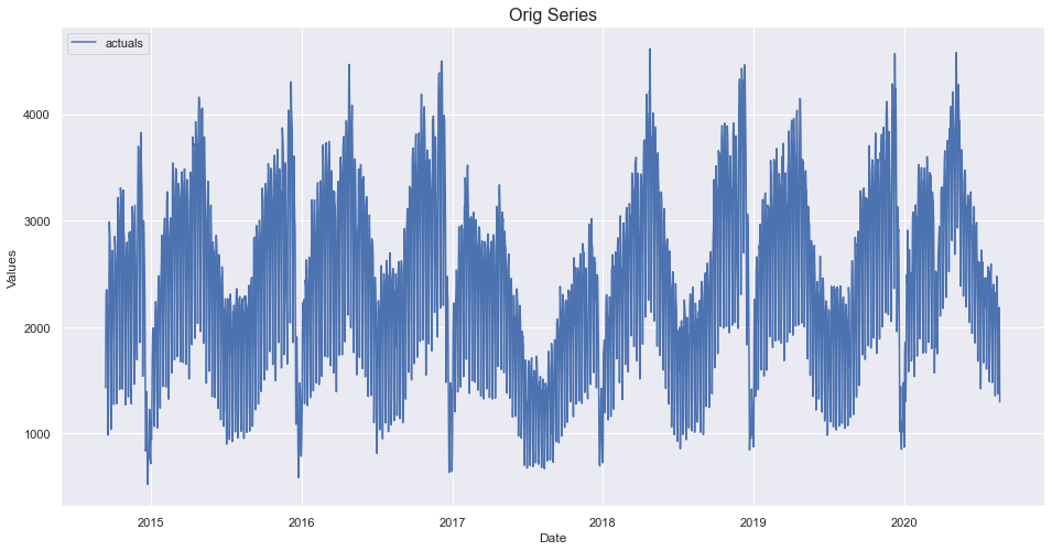
f=Forecaster(y=data['First.Time.Visits'],current_dates=data['Date'])
f.plot()
plt.title('Orig Series',size=16)
plt.show()

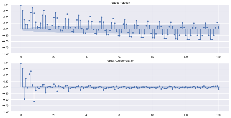
figs, axs = plt.subplots(2, 1)
f.plot_acf(ax=axs[0],lags=120)
f.plot_pacf(ax=axs[1],lags=120)
plt.show()

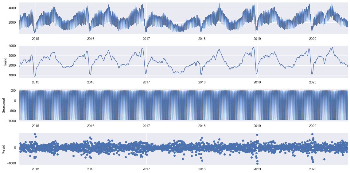
f.seasonal_decompose().plot()
plt.show()

ADF Test

critical_pval = 0.05
print('-'*100)
print('Augmented Dickey-Fuller results:')
stat, pval, _, _, _, _ = f.adf_test(full_res=True)
print('the test-stat value is: {:.2f}'.format(stat))
print('the p-value is {:.4f}'.format(pval))
print('the series is {}'.format('stationary' if pval < critical_pval else 'not stationary'))
print('-'*100)

----------------------------------------------------------------------------------------------------
Augmented Dickey-Fuller results:
the test-stat value is: -4.48
the p-value is 0.0002
the series is stationary
----------------------------------------------------------------------------------------------------

Preparing the data for modeling

f.generate_future_dates(60)
f.set_test_length(.2)
f.set_estimator('prophet')
f

Forecaster(
    DateStartActuals=2014-09-14T00:00:00.000000000
    DateEndActuals=2020-08-19T00:00:00.000000000
    Freq=D
    N_actuals=2167
    ForecastLength=60
    Xvars=[]
    Differenced=0
    TestLength=433
    ValidationLength=1
    ValidationMetric=rmse
    ForecastsEvaluated=[]
    CILevel=0.95
    BootstrapSamples=100
    CurrentEstimator=prophet
)

Forecasting

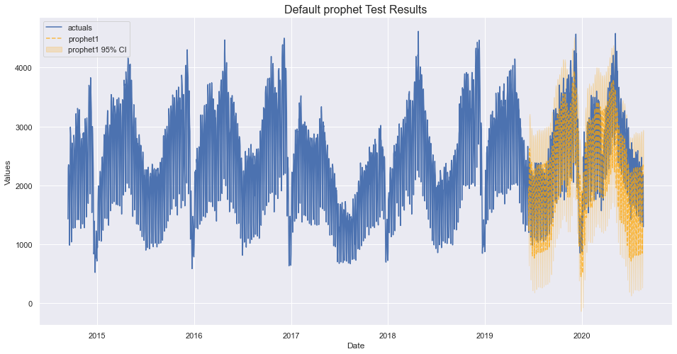
f.manual_forecast(call_me='prophet1')

f.plot_test_set(ci=True,models='prophet1')
plt.title('Default prophet Test Results',size=16)
plt.show()

results = f.export('model_summaries')
results[['TestSetRMSE','InSampleRMSE','TestSetMAPE','InSampleMAPE']]

	TestSetRMSE	InSampleRMSE	TestSetMAPE	InSampleMAPE
0	403.968233	283.145403	0.136388	0.104243

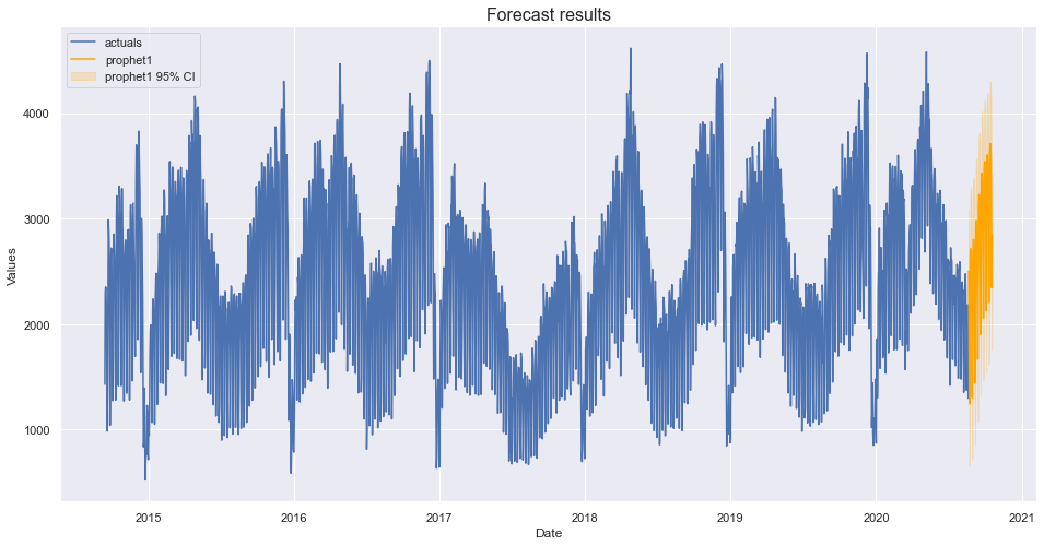
f.plot(ci=True,models='prophet1')
plt.title('Forecast results',size=16)
plt.show()