Validation

There are many ways to validate a model with scalecast and this notebook introduces them and overviews the differences between dynamic and non-dynamic tuning/testing, cross-validation, backtesting, and the eye test.

• Download data: https://www.kaggle.com/robervalt/sunspots

• See here for EDA on this dataset: https://scalecast-examples.readthedocs.io/en/latest/rnn/rnn.html

• See here for documentation on cross validation: https://scalecast.readthedocs.io/en/latest/Forecaster/Forecaster.html#src.scalecast.Forecaster.Forecaster.cross_validate

import pandas as pd
import numpy as np
import matplotlib.pyplot as plt
import seaborn as sns
from scalecast.Forecaster import Forecaster
import diagram_creator

def prepare_fcst(f, test_length=0.1, fcst_length=120):
    """ adds all variables and sets the test length/forecast length in the object

    Args:
        f (Forecaster): the Forecaster object.
        test_length (int or float): the test length as a size or proportion.
        fcst_length (int): the forecast horizon.

    Returns:
        (Forecaster) the processed object.
    """
    f.generate_future_dates(fcst_length)
    f.set_test_length(test_length)
    f.set_validation_length(f.test_length)
    f.eval_cis()
    f.add_seasonal_regressors("month")
    for i in np.arange(60, 289, 12):  # 12-month cycles from 12 to 288 months
        f.add_cycle(i)
    f.add_ar_terms(120)  # AR 1-120
    f.add_AR_terms((20, 12))  # seasonal AR up to 20 years, spaced one year apart
    f.add_seasonal_regressors("year")
    #f.auto_Xvar_select(irr_cycles=[120],estimator='gbt')
    return f


def export_results(f):
    """ returns a dataframe with all model results given a Forecaster object.

    Args:
        f (Forecaster): the Forecaster object.

    Returns:
        (DataFrame) the dataframe with the pertinent results.
    """
    results = f.export("model_summaries", determine_best_by="TestSetMAE")
    return results[
        [
            "ModelNickname",
            "TestSetRMSE",
            "InSampleRMSE",
            "ValidationMetric",
            "ValidationMetricValue",
            "HyperParams",
            "TestSetLength",
            "DynamicallyTested",
        ]
    ]

Load Forecaster Object

• we choose 120 periods (10 years) for all validation and forecasting

• 10 years of observervations to tune model hyperparameters, 10 years to test, and a forecast horizon of 10 years

df = pd.read_csv("Sunspots.csv", index_col=0, names=["Date", "Target"], header=0)
f = Forecaster(y=df["Target"], current_dates=df["Date"])
prepare_fcst(f)

Forecaster(
    DateStartActuals=1749-01-31T00:00:00.000000000
    DateEndActuals=2021-01-31T00:00:00.000000000
    Freq=M
    N_actuals=3265
    ForecastLength=120
    Xvars=['month', 'cycle60sin', 'cycle60cos', 'cycle72sin', 'cycle72cos', 'cycle84sin', 'cycle84cos', 'cycle96sin', 'cycle96cos', 'cycle108sin', 'cycle108cos', 'cycle120sin', 'cycle120cos', 'cycle132sin', 'cycle132cos', 'cycle144sin', 'cycle144cos', 'cycle156sin', 'cycle156cos', 'cycle168sin', 'cycle168cos', 'cycle180sin', 'cycle180cos', 'cycle192sin', 'cycle192cos', 'cycle204sin', 'cycle204cos', 'cycle216sin', 'cycle216cos', 'cycle228sin', 'cycle228cos', 'cycle240sin', 'cycle240cos', 'cycle252sin', 'cycle252cos', 'cycle264sin', 'cycle264cos', 'cycle276sin', 'cycle276cos', 'cycle288sin', 'cycle288cos', 'AR1', 'AR2', 'AR3', 'AR4', 'AR5', 'AR6', 'AR7', 'AR8', 'AR9', 'AR10', 'AR11', 'AR12', 'AR13', 'AR14', 'AR15', 'AR16', 'AR17', 'AR18', 'AR19', 'AR20', 'AR21', 'AR22', 'AR23', 'AR24', 'AR25', 'AR26', 'AR27', 'AR28', 'AR29', 'AR30', 'AR31', 'AR32', 'AR33', 'AR34', 'AR35', 'AR36', 'AR37', 'AR38', 'AR39', 'AR40', 'AR41', 'AR42', 'AR43', 'AR44', 'AR45', 'AR46', 'AR47', 'AR48', 'AR49', 'AR50', 'AR51', 'AR52', 'AR53', 'AR54', 'AR55', 'AR56', 'AR57', 'AR58', 'AR59', 'AR60', 'AR61', 'AR62', 'AR63', 'AR64', 'AR65', 'AR66', 'AR67', 'AR68', 'AR69', 'AR70', 'AR71', 'AR72', 'AR73', 'AR74', 'AR75', 'AR76', 'AR77', 'AR78', 'AR79', 'AR80', 'AR81', 'AR82', 'AR83', 'AR84', 'AR85', 'AR86', 'AR87', 'AR88', 'AR89', 'AR90', 'AR91', 'AR92', 'AR93', 'AR94', 'AR95', 'AR96', 'AR97', 'AR98', 'AR99', 'AR100', 'AR101', 'AR102', 'AR103', 'AR104', 'AR105', 'AR106', 'AR107', 'AR108', 'AR109', 'AR110', 'AR111', 'AR112', 'AR113', 'AR114', 'AR115', 'AR116', 'AR117', 'AR118', 'AR119', 'AR120', 'AR132', 'AR144', 'AR156', 'AR168', 'AR180', 'AR192', 'AR204', 'AR216', 'AR228', 'AR240', 'year']
    TestLength=326
    ValidationMetric=rmse
    ForecastsEvaluated=[]
    CILevel=0.95
    CurrentEstimator=mlr
    GridsFile=Grids
)

f.set_estimator('gbt')

In the feature_selection notebook, gbt was chosen as the best model class out of several tried. We will show all examples with this estimator.

Default Model Parameters

• one with dynamic testing

• one with non-dynamic testing

• the difference can be expressed by taking the case of a simple autoregressive model, such that:

Non-Dynamic Autoregressive Predictions

\[x_t = \alpha * x_{t-1} + e_t\]

Over an indefinite forecast horizon, the above equation would only work if you knew the value for \(x_{t-1}\). Going more than one period into the future, you would stop knowing what that value is. In a test-set of data, of course, you do know all values into the forecast horizon, but to be more realistic, you could write an equation for a two-step forecast like this:

Dynamic Autoregressive Predictions

\[\hat{x_t} = \hat{\alpha} * x_{t-1}\]

\[x_{t+1} = \hat{\alpha} * \hat{x}_t + e_{t+1}\]

Using these two equations, which scalecast refers to as dynamic forecasting, you could evaluate any forecast horizon by plugging in predicted values for \(x_{t-1}\) or \({x_t}\) over periods in which you did not know it. This is default behavior for all models tested through scalecast, but it is not default for tuning models. We will explore dynamic tuning soon. First, let’s see in practical terms the difference between non-dynamic and dynamic testing.

f.manual_forecast(call_me="gbt_default_non-dynamic", dynamic_testing=False)
f.manual_forecast(call_me="gbt_default_dynamic")  # default is dynamic testing

f.plot_test_set(
    models=[
        "gbt_default_non-dynamic",
        "gbt_default_dynamic"
    ],
    include_train=False,
)
plt.show()

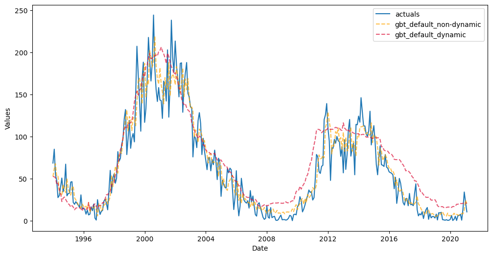
It appears that the non-dynamically tested model performed significantly better than the other, but looks can be deceiving. In essence, the non-dynamic model was only tested for its ability to perform 326 one-step forecasts and its final metric is an average of these one-step forecasts. It could be a good idea to set dynamic_testing=False if you want to speed up the testing process or if you only care about how your model would perform one step into the future. But to report the test-set metric from this model as if it could be expected to do that well for the full 326 periods into the future is misleading. The other model that was dynamically tested can be more realistically trusted in that regard.

export_results(f)

	ModelNickname	TestSetRMSE	InSampleRMSE	ValidationMetric	ValidationMetricValue	HyperParams	TestSetLength	DynamicallyTested
0	gbt_default_non-dynamic	18.723179	18.841544	NaN	NaN	{}	326	False
1	gbt_default_dynamic	24.456923	18.841544	NaN	NaN	{}	326	True

Tune the model to find optimal hyperparameters

• Create a validation grid

• Try three strategies to tune the parameters:

• Train/validation/test split

  • Hyperparameters are tried on the validation set

• Train/test split with 5-fold time-series cross-validation on training set

  • Training data split 5 times into train/validations set

  • Models trained on training set only

  • Validated out-of-sample

  • All data available before each validation split sequentially used to train the model

• Train/test split with 5-fold time-series rolling cross-validation on training set

  • Rolling is different in that each train/validation split is the same size

grid = {
    "max_depth": [2, 3, 5],
    "max_features": ["sqrt", "auto"],
    "subsample": [0.8, 0.9, 1],
}

f.ingest_grid(grid)

Train/Validation/Test Split

• The data’s sequence is always maintained in time-series splits with scalecast

f.tune(dynamic_tuning=True)
f.auto_forecast(
    call_me="gbt_tuned"
)  # automatically uses optimal paramaeters suggested from the tuning process

f.export_validation_grid("gbt_tuned").sort_values('AverageMetric').head(10)

	max_depth	max_features	subsample	Fold0Metric	AverageMetric	MetricEvaluated
7	3	sqrt	0.9	43.623057	43.623057	rmse
12	5	sqrt	0.8	43.667072	43.667072	rmse
6	3	sqrt	0.8	44.015361	44.015361	rmse
8	3	sqrt	1	44.807485	44.807485	rmse
0	2	sqrt	0.8	46.093143	46.093143	rmse
2	2	sqrt	1	53.206496	53.206496	rmse
14	5	sqrt	1	60.587243	60.587243	rmse
10	3	auto	0.9	65.424393	65.424393	rmse
15	5	auto	0.8	66.530315	66.530315	rmse
13	5	sqrt	0.9	67.459775	67.459775	rmse

5-Fold Time Series Cross Validation

• Split training set into k (5) folds

• Each validation set is the same size and determined such that: val_size = n_obs // (folds + 1)

• The last training set will be the same size or almost the same size as the validation sets

• Model trained and re-trained with all data that came before each validation slice

• Each fold tested out of sample on its validation set

• Final error is an average of the out-of-sample error obtained from each fold

• The chosen hyperparameters are determined by which final error was minimized

• Below is an example with a dataset sized 100 observations and in which 10 observations are held out for testing and the remaining 90 observations are used as the training set:

diagram_creator.create_cv()

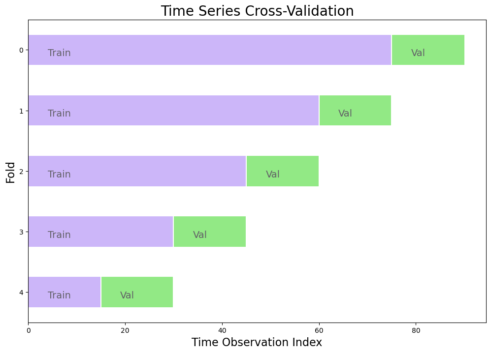
The final error, E, can be expressed as an average of the error from each fold i:

\[E = \frac{1}{n}\sum_{i=0}^{n-1}{(e_i)}\]

f.cross_validate(
    k=5,
    dynamic_tuning=True,
    test_length = None, # default so that last test and train sets are same size (or close to the same)
    train_length = None, # default uses all observations before each test set
    space_between_sets = None, # default adds a length equal to the test set between consecutive sets
    verbose = True, # print out info about each fold
)
f.auto_forecast(call_me="gbt_cv")

Num hyperparams to try for the gbt model: 18.
Fold 0: Train size: 2450 (1749-01-31 00:00:00 - 1953-02-28 00:00:00). Test Size: 489 (1953-03-31 00:00:00 - 1993-11-30 00:00:00).
Fold 1: Train size: 1961 (1749-01-31 00:00:00 - 1912-05-31 00:00:00). Test Size: 489 (1912-06-30 00:00:00 - 1953-02-28 00:00:00).
Fold 2: Train size: 1472 (1749-01-31 00:00:00 - 1871-08-31 00:00:00). Test Size: 489 (1871-09-30 00:00:00 - 1912-05-31 00:00:00).
Fold 3: Train size: 983 (1749-01-31 00:00:00 - 1830-11-30 00:00:00). Test Size: 489 (1830-12-31 00:00:00 - 1871-08-31 00:00:00).
Fold 4: Train size: 494 (1749-01-31 00:00:00 - 1790-02-28 00:00:00). Test Size: 489 (1790-03-31 00:00:00 - 1830-11-30 00:00:00).
Chosen paramaters: {'max_depth': 5, 'max_features': 'sqrt', 'subsample': 1}.

f.export_validation_grid("gbt_cv").sort_values("AverageMetric").head(10)

	max_depth	max_features	subsample	Fold0Metric	Fold1Metric	Fold2Metric	Fold3Metric	Fold4Metric	AverageMetric	MetricEvaluated
14	5	sqrt	1	75.881634	85.585377	79.162305	83.264294	96.912215	84.161165	rmse
12	5	sqrt	0.8	90.328729	96.703967	48.606034	80.703070	111.586242	85.585609	rmse
13	5	sqrt	0.9	108.327532	95.594713	61.082475	61.798101	108.437289	87.048022	rmse
16	5	auto	0.9	89.047882	92.811981	74.332318	86.321627	112.510827	91.004927	rmse
0	2	sqrt	0.8	105.541098	78.227464	103.386493	77.997451	115.573720	96.145245	rmse
8	3	sqrt	1	64.668019	119.509341	93.877028	93.740770	114.533147	97.265661	rmse
7	3	sqrt	0.9	75.061438	85.898970	122.575339	91.157722	119.005642	98.739822	rmse
2	2	sqrt	1	59.907395	88.529044	113.535870	118.721240	117.856393	99.709989	rmse
17	5	auto	1	111.676983	96.506098	70.688360	102.882864	118.365703	100.024002	rmse
6	3	sqrt	0.8	93.640946	85.464725	100.451257	109.813079	111.415691	100.157140	rmse

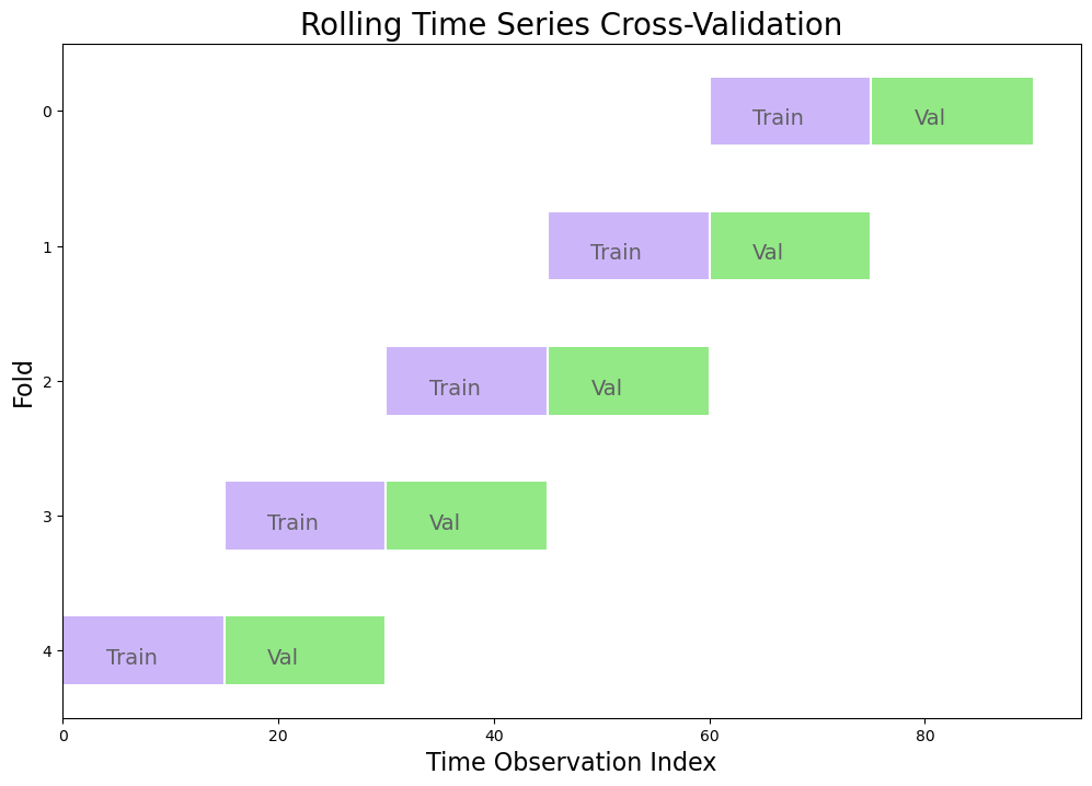
5-Fold Rolling Time Series Cross Validation

• Split training set into k (5) folds

• Each validation set is the same size

• Each training set is also the same size as each validation set

• Each fold tested out of sample

• Final error is an average of the out-of-sample error obtained from each folds

• The chosen hyperparameters are determined by which final error was minimized

• Below is an example with a dataset sized 100 observation and in which 10 observations are held out for testing and the remaining 90 observations are used as the training set:

diagram_creator.create_rolling_cv()

f.cross_validate(
    k=5,
    rolling=True,
    dynamic_tuning=True,
    test_length = None, # with rolling = True, makes all train and test sets the same size
    train_length = None, # with rolling = True, makes all train and test sets the same size
    space_between_sets = None, # default adds a length equal to the test set between consecutive sets
    verbose = True, # print out info about each fold
)
f.auto_forecast(call_me="gbt_rolling_cv")

Num hyperparams to try for the gbt model: 18.
Fold 0: Train size: 489 (1912-06-30 00:00:00 - 1953-02-28 00:00:00). Test Size: 489 (1953-03-31 00:00:00 - 1993-11-30 00:00:00).
Fold 1: Train size: 489 (1871-09-30 00:00:00 - 1912-05-31 00:00:00). Test Size: 489 (1912-06-30 00:00:00 - 1953-02-28 00:00:00).
Fold 2: Train size: 489 (1830-12-31 00:00:00 - 1871-08-31 00:00:00). Test Size: 489 (1871-09-30 00:00:00 - 1912-05-31 00:00:00).
Fold 3: Train size: 489 (1790-03-31 00:00:00 - 1830-11-30 00:00:00). Test Size: 489 (1830-12-31 00:00:00 - 1871-08-31 00:00:00).
Fold 4: Train size: 489 (1749-06-30 00:00:00 - 1790-02-28 00:00:00). Test Size: 489 (1790-03-31 00:00:00 - 1830-11-30 00:00:00).
Chosen paramaters: {'max_depth': 5, 'max_features': 'sqrt', 'subsample': 0.9}.

f.export_validation_grid("gbt_rolling_cv").sort_values("AverageMetric").head(10)

	max_depth	max_features	subsample	Fold0Metric	Fold1Metric	Fold2Metric	Fold3Metric	Fold4Metric	AverageMetric	MetricEvaluated
13	5	sqrt	0.9	52.067612	75.101589	47.665446	73.458303	110.673685	71.793327	rmse
11	3	auto	1	61.780860	70.554830	48.914548	74.467054	110.351684	73.213795	rmse
9	3	auto	0.8	59.526670	76.807231	48.096324	74.276742	110.628222	73.867038	rmse
17	5	auto	1	68.884924	63.475008	52.178487	73.895434	111.100209	73.906812	rmse
7	3	sqrt	0.9	44.798329	69.131312	54.226665	93.287371	115.134538	75.315643	rmse
8	3	sqrt	1	56.409051	84.081666	49.339527	75.453036	111.791536	75.414963	rmse
3	2	auto	0.8	61.498220	73.383101	48.898466	78.773421	115.272207	75.565083	rmse
12	5	sqrt	0.8	63.732031	78.140692	47.053796	73.473322	115.558499	75.591668	rmse
5	2	auto	1	69.075181	67.852121	53.383812	75.150129	115.413148	76.174878	rmse
14	5	sqrt	1	48.860162	84.807936	49.921226	89.144401	110.995682	76.745881	rmse

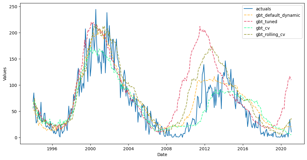
View results

f.plot_test_set(
    models=[
        "gbt_default_dynamic",
        "gbt_tuned",
        "gbt_cv",
        "gbt_rolling_cv",
    ],
    include_train=False,
)
plt.show()

pd.set_option('max_colwidth', 60)
export_results(f)

	ModelNickname	TestSetRMSE	InSampleRMSE	ValidationMetric	ValidationMetricValue	HyperParams	TestSetLength	DynamicallyTested
0	gbt_default_non-dynamic	18.723179	18.841544	NaN	NaN	{}	326	False
1	gbt_default_dynamic	24.456923	18.841544	NaN	NaN	{}	326	True
2	gbt_cv	25.604943	13.063379	rmse	84.161165	{'max_depth': 5, 'max_features': 'sqrt', 'subsample': 1}	326	True
3	gbt_rolling_cv	34.248137	12.789779	rmse	71.793327	{'max_depth': 5, 'max_features': 'sqrt', 'subsample': 0.9}	326	True
4	gbt_tuned	50.777958	20.342340	rmse	43.623057	{'max_depth': 3, 'max_features': 'sqrt', 'subsample': 0.9}	326	True

Backtest models

• Backtesting is a process in which the final chosen model is re-validated by seeing its average performance on the last x-number of forecast horizons available in the data

• With scalecast, pipeline objects can be built and backtest all applied models to see the best one over several forecast horizons

• See the documentation for more information

from scalecast.Pipeline import Pipeline
from scalecast.util import backtest_metrics

def forecaster(f):
    f.set_estimator('gbt')
    f.set_validation_length(int(len(f.y)*.1)) # 10% val length each time
    f.add_seasonal_regressors("month")
    for i in np.arange(60, 289, 12):  # 12-month cycles from 12 to 288 months
        f.add_cycle(i)
    f.add_ar_terms(120)  # AR 1-120
    f.add_AR_terms((20, 12))  # seasonal AR up to 20 years, spaced one year apart
    f.add_seasonal_regressors("year")

    f.manual_forecast(call_me='gbt_default_dynamic')

    f.ingest_grid(grid)

    f.tune(dynamic_tuning = True)
    f.auto_forecast(call_me='gbt_tuned')

    f.cross_validate(dynamic_tuning = True)
    f.auto_forecast(call_me='gbt_cv')

    f.cross_validate(dynamic_tuning = True, rolling = True)
    f.auto_forecast(call_me='gbt_rolling_cv')

pipeline = Pipeline(steps = [('Forecast',forecaster)])

backtest_results = pipeline.backtest(
    f,
    test_length = 0,
    fcst_length = 120,
    jump_back = 120, # place 120 obs between each training set
    cis = False,
    verbose = True,
)

bm = backtest_metrics(backtest_results,mets=['rmse','mae','r2'])
bm

		Iter0	Iter1	Iter2	Iter3	Iter4	Average
Model	Metric
gbt_default_dynamic	rmse	29.787489	32.631984	40.218024	57.655588	88.550393	49.768696
	mae	24.725663	25.120353	32.70369	45.658795	56.387906	36.919281
	r2	0.499971	0.718315	0.652106	0.466619	-0.415585	0.384285
gbt_tuned	rmse	21.793363	38.201181	34.145031	55.637363	99.862839	49.927956
	mae	17.232072	29.314773	26.055781	42.62898	63.122565	35.670834
	r2	0.732345	0.613962	0.749239	0.503307	-0.800374	0.359696
gbt_cv	rmse	27.290614	30.871908	38.859572	55.141773	35.648112	37.562396
	mae	21.956079	24.026144	30.078019	42.157045	27.85357	29.214172
	r2	0.580286	0.747883	0.675211	0.512116	0.770582	0.657215
gbt_rolling_cv	rmse	26.080319	31.8572	34.485633	43.732603	38.312404	34.893632
	mae	21.003643	24.701014	27.536833	37.057153	28.484026	27.756534
	r2	0.616687	0.731533	0.744211	0.693122	0.735007	0.704112

bmr = bm.reset_index()

bmrrmse = bmr.loc[bmr['Metric'] == 'rmse'].sort_values('Average')
best_model = bmrrmse.iloc[0,0]
best_model

'gbt_rolling_cv'

rmse = bmr.loc[
    (bmr['Model'] == best_model) & (bmr['Metric'] == 'rmse'),
    'Average',
].values[0]
mae = bmr.loc[
    (bmr['Model'] == best_model) & (bmr['Metric'] == 'mae'),
    'Average',
].values[0]
r2 = bmr.loc[
    (bmr['Model'] == best_model) & (bmr['Metric'] == 'r2'),
    'Average',
].values[0]

print(
    f"The best model, according to the RMSE over 5 backtest iterations was {best_model}."
    " On average, we can expect this model to have an RMSE of"
    f" {rmse:.2f}, MAE of {mae:.2f}, and R2 of {r2:.2%} over a full 120-period"
    " forecast window."
)

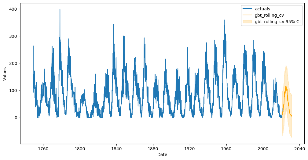
The best model, according to the RMSE over 5 backtest iterations was gbt_rolling_cv. On average, we can expect this model to have an RMSE of 34.89, MAE of 27.76, and R2 of 70.41% over a full 120-period forecast window.

An extension of this analysis could be to choose regressors more carefully (see here) and to use more complex models (see here).

The Eye Test

In addition to all the objective validation performed in this notebook, one of the most important questions to ask is if the forecast looks reasonable. Does it pass the common sense test? Below, we plot the 120-forecast period horizon from the best model.

f.plot(models=best_model, ci = True)
plt.show()