Transfer Learning - TensorFlow

• Transfer learning tensorflow (RNN/LSTM) models works slightly different than other model types, due to the difficulty of carrying these models in Forecaster object history. Forecater objects are meant to be be copied and pickled, both of which can fail with tensorflow models. For that reason, it is good to save out tensorflow models manually before using them to transfer learn.

• This notebook also demonstrates transferring confidence intervals.

• Requires >=0.19.1.

from scalecast.Forecaster import Forecaster
from scalecast.util import infer_apply_Xvar_selection, find_optimal_transformation
from scalecast.Pipeline import Pipeline, Transformer, Reverter
from scalecast import GridGenerator
import pandas_datareader as pdr
import matplotlib.pyplot as plt
import pandas as pd

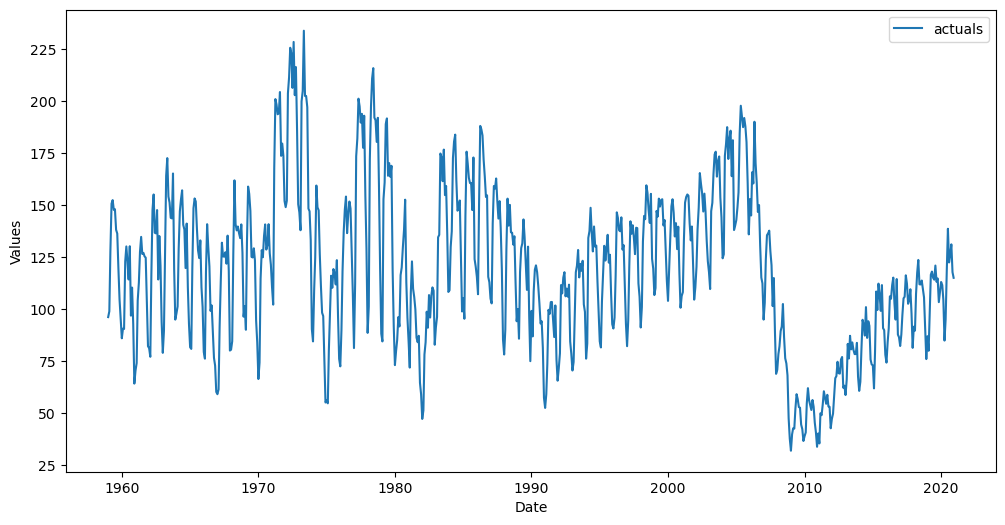
Initiate the First Forecaster Object

This series ends December, 2020.

df = pdr.get_data_fred(
    'HOUSTNSA',
    start = '1959-01-01',
    end = '2020-12-31',
)

df.head()

	HOUSTNSA
DATE
1959-01-01	96.2
1959-02-01	99.0
1959-03-01	127.7
1959-04-01	150.8
1959-05-01	152.5

f = Forecaster(
    y = df.iloc[:,0],
    current_dates = df.index,
    future_dates = 24,
    cis=True,
    test_length = 24,
)

f.plot()
plt.show()

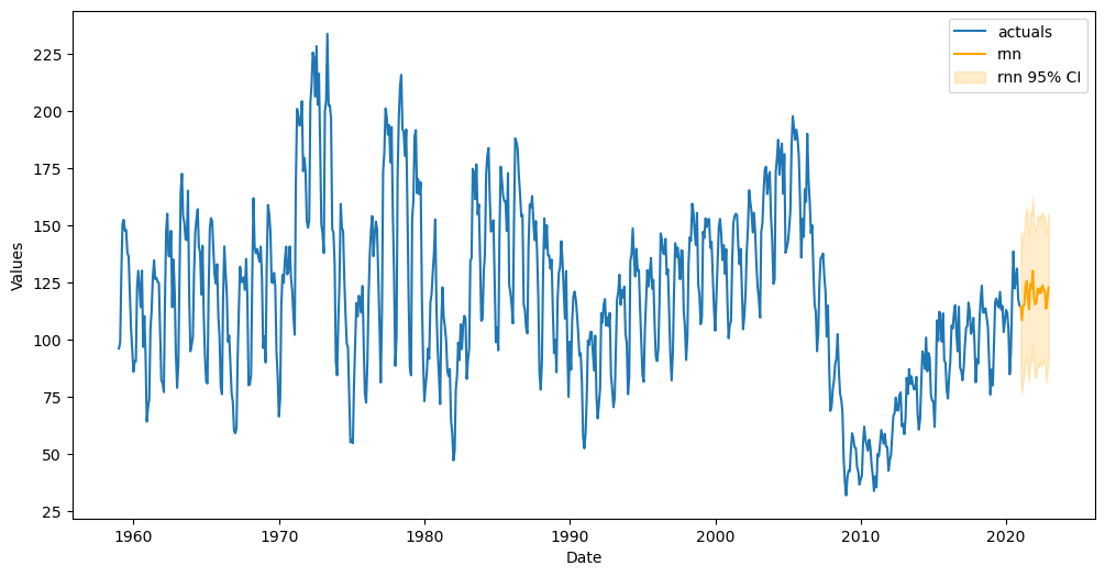
Fit the RNN Model

f.set_estimator('rnn')
f.manual_forecast(epochs=15,lags=24)

Epoch 1/15
21/21 [==============================] - 2s 8ms/step - loss: 0.4615
Epoch 2/15
21/21 [==============================] - 0s 9ms/step - loss: 0.3677
Epoch 3/15
21/21 [==============================] - 0s 8ms/step - loss: 0.2878
Epoch 4/15
21/21 [==============================] - 0s 8ms/step - loss: 0.2330
Epoch 5/15
21/21 [==============================] - 0s 8ms/step - loss: 0.1968
Epoch 6/15
21/21 [==============================] - 0s 8ms/step - loss: 0.1724
Epoch 7/15
21/21 [==============================] - 0s 8ms/step - loss: 0.1555
Epoch 8/15
21/21 [==============================] - 0s 7ms/step - loss: 0.1454
Epoch 9/15
21/21 [==============================] - 0s 7ms/step - loss: 0.1393
Epoch 10/15
21/21 [==============================] - 0s 8ms/step - loss: 0.1347
Epoch 11/15
21/21 [==============================] - 0s 7ms/step - loss: 0.1323
Epoch 12/15
21/21 [==============================] - 0s 7ms/step - loss: 0.1303
Epoch 13/15
21/21 [==============================] - 0s 6ms/step - loss: 0.1279
Epoch 14/15
21/21 [==============================] - 0s 7ms/step - loss: 0.1275
Epoch 15/15
21/21 [==============================] - 0s 7ms/step - loss: 0.1261
1/1 [==============================] - 0s 345ms/step
Epoch 1/15
22/22 [==============================] - 2s 8ms/step - loss: 0.3696
Epoch 2/15
22/22 [==============================] - 0s 7ms/step - loss: 0.3072
Epoch 3/15
22/22 [==============================] - 0s 6ms/step - loss: 0.2600
Epoch 4/15
22/22 [==============================] - 0s 6ms/step - loss: 0.2255
Epoch 5/15
22/22 [==============================] - 0s 6ms/step - loss: 0.2014
Epoch 6/15
22/22 [==============================] - 0s 6ms/step - loss: 0.1840
Epoch 7/15
22/22 [==============================] - 0s 5ms/step - loss: 0.1713
Epoch 8/15
22/22 [==============================] - 0s 5ms/step - loss: 0.1616
Epoch 9/15
22/22 [==============================] - 0s 5ms/step - loss: 0.1557
Epoch 10/15
22/22 [==============================] - 0s 5ms/step - loss: 0.1503
Epoch 11/15
22/22 [==============================] - 0s 5ms/step - loss: 0.1437
Epoch 12/15
22/22 [==============================] - 0s 6ms/step - loss: 0.1404
Epoch 13/15
22/22 [==============================] - 0s 5ms/step - loss: 0.1381
Epoch 14/15
22/22 [==============================] - 0s 6ms/step - loss: 0.1354
Epoch 15/15
22/22 [==============================] - 0s 6ms/step - loss: 0.1339
1/1 [==============================] - 0s 327ms/step
22/22 [==============================] - 0s 3ms/step

f.plot(ci=True)
plt.show()

Save the model out

After you fit a tensforflow model, the fit model is attached to the Forecaster in the tf_model attribute. You can view the model summary:

f.tf_model.summary()

Model: "sequential_1"
_________________________________________________________________
 Layer (type)                Output Shape              Param #
=================================================================
 simple_rnn_1 (SimpleRNN)    (None, 8)                 80

 dense_1 (Dense)             (None, 24)                216

=================================================================
Total params: 296
Trainable params: 296
Non-trainable params: 0
_________________________________________________________________

However, immediately after changing estimators or when the object is pickled out, this attribute is lost. Therefore, it is a good idea to save the model out:

f.save_tf_model(name='model.h5') # default argument

Later, when you want to transfer learn with the model, you can re-attach it to the Forecaster object:

f.load_tf_model(name='model.h5') # default argument

This re-attaches the tf_model attribute.

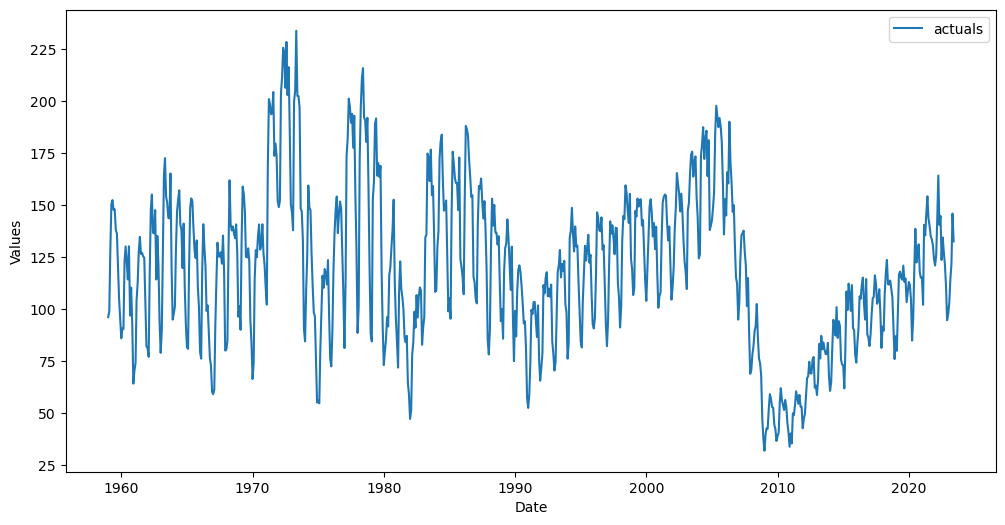
Initiate the Second Forecaster Object

• Later, if we have more data streaming in, instead of refitting a model, we can use the already-fitted model to make the predictions. This updated series is through June, 2023

• You can use an updated version of the original series, you can use the same series with an extended Forecast horizon, or you can use an entirely different series (as long as it’s the same frequency) to perform this process

df_new = pdr.get_data_fred(
    'HOUSTNSA',
    start = '1959-01-01',
    end = '2023-06-30',
)

df_new.tail()

	HOUSTNSA
DATE
2023-02-01	103.2
2023-03-01	114.0
2023-04-01	121.7
2023-05-01	146.0
2023-06-01	132.6

f_new = Forecaster(
    y = df_new.iloc[:,0],
    current_dates = df_new.index,
    future_dates = 24,
)

f_new.plot()
plt.show()

Add the same Xvars to the new Forecaster object

• The helper function below can assist when you automatically added Xvars

• If you manually added Xvars, you can wrap the selection process in a function and run this new Forecaster object through the same function.

infer_apply_Xvar_selection(infer_from=f,apply_to=f_new)

Forecaster(
    DateStartActuals=1959-01-01T00:00:00.000000000
    DateEndActuals=2023-06-01T00:00:00.000000000
    Freq=MS
    N_actuals=774
    ForecastLength=24
    Xvars=['AR1', 'AR2', 'AR3', 'AR4', 'AR5', 'AR6', 'AR7', 'AR8', 'AR9', 'AR10', 'AR11', 'AR12', 'AR13', 'AR14', 'AR15', 'AR16', 'AR17', 'AR18', 'AR19', 'AR20', 'AR21', 'AR22', 'AR23', 'AR24']
    TestLength=0
    ValidationMetric=rmse
    ForecastsEvaluated=[]
    CILevel=None
    CurrentEstimator=mlr
    GridsFile=Grids
)

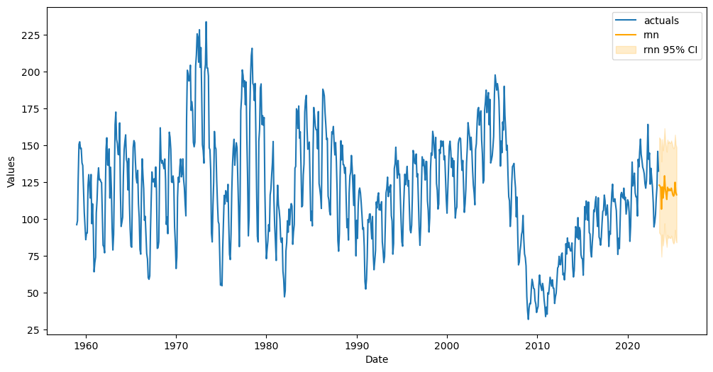
Apply fitted model from first object onto this new object

f_new.transfer_predict(transfer_from=f,model='rnn',model_type='tf')

1/1 [==============================] - 0s 149ms/step
23/23 [==============================] - 0s 2ms/step

Transfer the model’s confidence intervals

f_new.transfer_cis(transfer_from=f,model='rnn') # transfer the model's confidence intervals

f_new.plot(ci=True)
plt.show()