Transfer Learning

• This notebook shows how to use one fitted model stored in a Forecaster object to make predictions on a separate time series.

• Requires >=0.19.0

• As of 0.19.1, univariate sklearn and tensorflow (RNN/LSTM) models are supported for this type of process. Multivariate sklearn, then the rest of the model types will be worked on next.

• See the documentation.

from scalecast.Forecaster import Forecaster
from scalecast.util import infer_apply_Xvar_selection, find_optimal_transformation
from scalecast.Pipeline import Pipeline, Transformer, Reverter
from scalecast import GridGenerator
import pandas_datareader as pdr
import matplotlib.pyplot as plt
import pandas as pd

GridGenerator.get_example_grids()

Initiate the First Forecaster Object

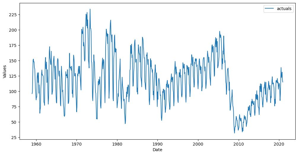
This series ends December, 2020.

df = pdr.get_data_fred(
    'HOUSTNSA',
    start = '1959-01-01',
    end = '2020-12-31',
)

df.tail()

	HOUSTNSA
DATE
2020-08-01	122.5
2020-09-01	126.3
2020-10-01	131.2
2020-11-01	117.8
2020-12-01	115.1

f = Forecaster(
    y = df.iloc[:,0],
    current_dates = df.index,
    future_dates = 24,
)

f.plot()
plt.show()

Automatically add Xvars to the object

f.auto_Xvar_select()
f

Forecaster(
    DateStartActuals=1959-01-01T00:00:00.000000000
    DateEndActuals=2020-12-01T00:00:00.000000000
    Freq=MS
    N_actuals=744
    ForecastLength=24
    Xvars=['AR1', 'AR2', 'AR3', 'AR4']
    TestLength=0
    ValidationMetric=rmse
    ForecastsEvaluated=[]
    CILevel=None
    CurrentEstimator=mlr
    GridsFile=Grids
)

Fit an XGBoost Model and Make Predictions

f.set_estimator('xgboost')
f.ingest_grid('xgboost')
f.limit_grid_size(10)
f.cross_validate(k=3,test_length=48)
f.auto_forecast()

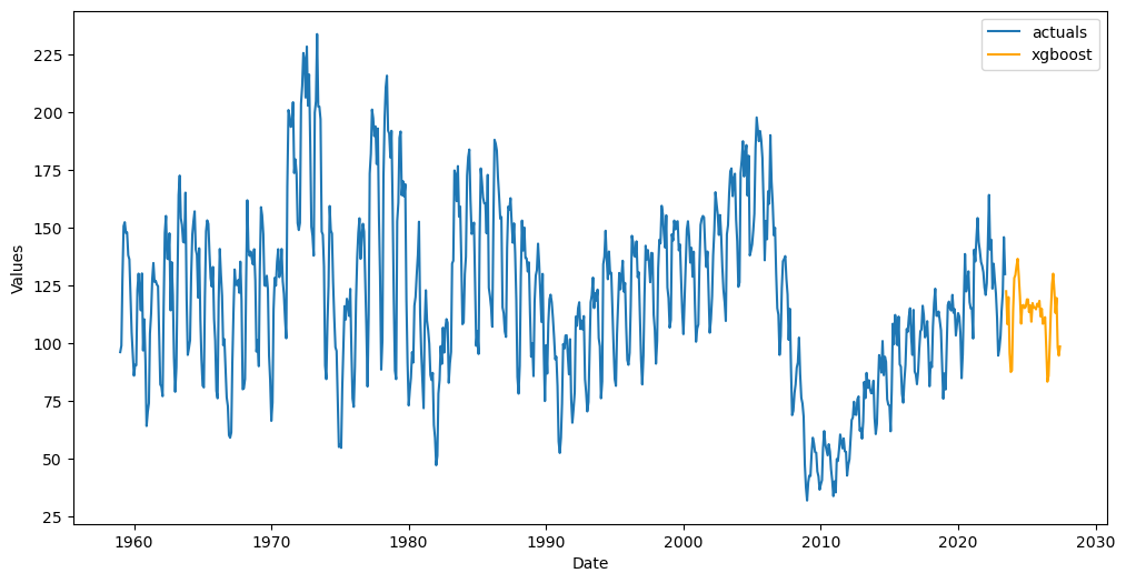
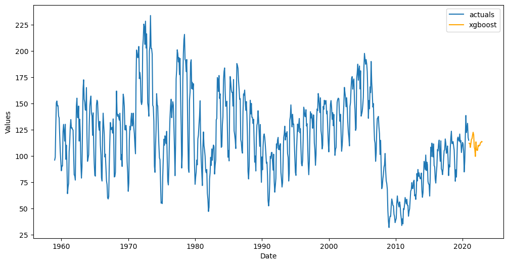
View the Forecast

f.plot()
plt.show()

Initiate the Second Forecaster Object

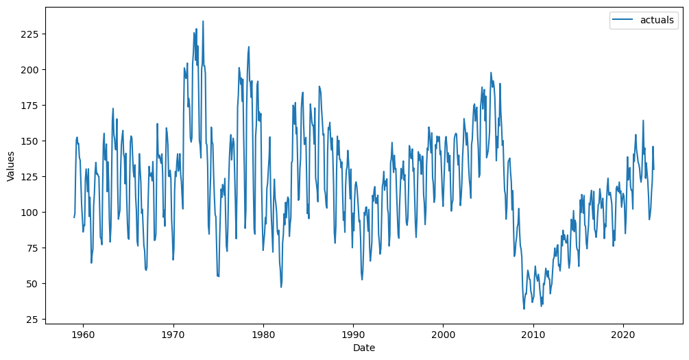
• Later, if we have more data streaming in, instead of refitting a model, we can use the already-fitted model to make the predictions. This updated series is through June, 2023

• You can use an updated version of the original series, you can use the same series with an extended Forecast horizon, or you can use an entirely different series (as long as it’s the same frequency) to perform this process

df_new = pdr.get_data_fred(
    'HOUSTNSA',
    start = '1959-01-01',
    end = '2023-06-30',
)

df_new.tail()

	HOUSTNSA
DATE
2023-02-01	103.2
2023-03-01	114.0
2023-04-01	121.7
2023-05-01	146.0
2023-06-01	130.0

f_new = Forecaster(
    y = df_new.iloc[:,0],
    current_dates = df_new.index,
    future_dates = 48,
)

f_new.plot()
plt.show()

Add the same Xvars to the new Forecaster object

• The helper function below can assist when you automatically added Xvars

• If you manually added Xvars, you can wrap the selection process in a function and run this new Forecaster object through the same function.

f_new = infer_apply_Xvar_selection(infer_from=f,apply_to=f_new)
f_new

Forecaster(
    DateStartActuals=1959-01-01T00:00:00.000000000
    DateEndActuals=2023-06-01T00:00:00.000000000
    Freq=MS
    N_actuals=774
    ForecastLength=48
    Xvars=['AR1', 'AR2', 'AR3', 'AR4']
    TestLength=0
    ValidationMetric=rmse
    ForecastsEvaluated=[]
    CILevel=None
    CurrentEstimator=mlr
    GridsFile=Grids
)

Apply fitted model from first object onto this new object

f_new.transfer_predict(transfer_from=f,model='xgboost')

View the new forecast

f_new.plot()
plt.show()

View the in-sample predictions

f_new.plot_fitted()
plt.show()

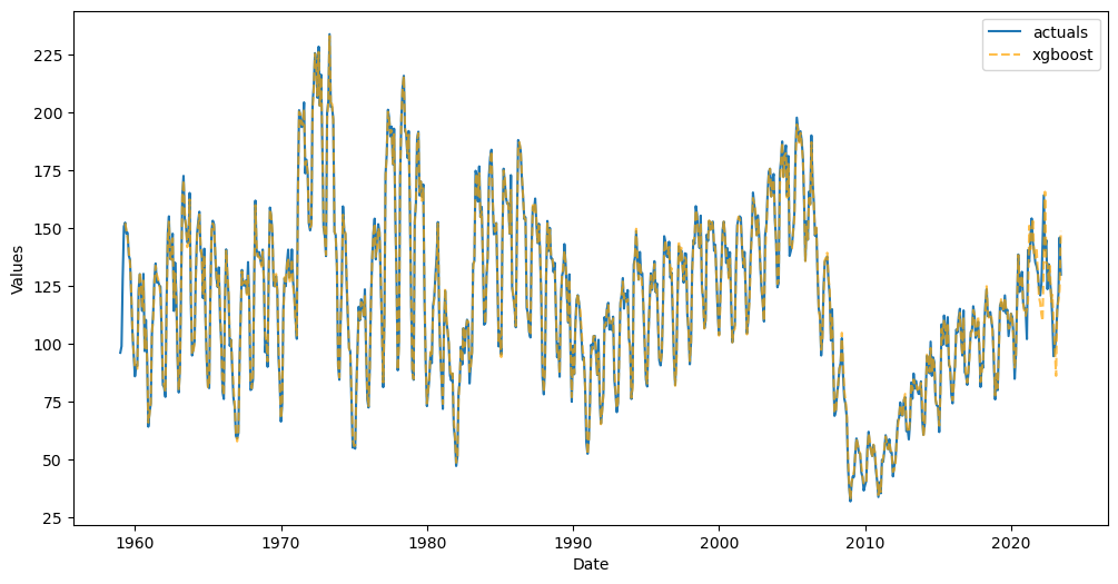
In the below plot, the model has seen all observations until December, 2020. From January, 2021 through June, 2023, it is seeing those observations for the first time, but because it has the actual y observations, its predictions are expected to be more accurate than the forecast into the unknown horizon.

Predict over a specific date range

• Instead of storing the model info into the new Forecaster object, you can instead get predicted output over a specific date range.

preds = f_new.transfer_predict(
    transfer_from = f,
    model = 'xgboost',
    dates = pd.date_range(start='2021-01-01',end='2023-12-31',freq='MS'),
    save_to_history=False,
    return_series=True,
)
preds

2021-01-01    112.175186
2021-02-01    115.029518
2021-03-01    118.659706
2021-04-01    151.111618
2021-05-01    140.886765
2021-06-01    147.894882
2021-07-01    154.100571
2021-08-01    137.926544
2021-09-01    137.189224
2021-10-01    141.547058
2021-11-01    130.737900
2021-12-01    120.278030
2022-01-01    117.764030
2022-02-01    112.886353
2022-03-01    110.008720
2022-04-01    139.413696
2022-05-01    165.805817
2022-06-01    135.017914
2022-07-01    134.379486
2022-08-01    126.559814
2022-09-01    133.788025
2022-10-01    118.278656
2022-11-01    121.269691
2022-12-01    110.270599
2023-01-01     98.168579
2023-02-01     86.210205
2023-03-01    115.844292
2023-04-01    118.449600
2023-05-01    123.620918
2023-06-01    148.793396
2023-07-01    122.571846
2023-08-01    108.331818
2023-09-01    120.023163
2023-10-01     95.729309
2023-11-01     87.593613
2023-12-01     88.265671
dtype: float32

From January through June, 2021, the predictions are considered in-sample, although the model has never previously seen them (it predicted using the actual y observations over that timespan, and that is a form of leakage for auto-regressive time series models). The rest of the predictions are truly out-of-sample.

Transfer Predict in a Pipeline

• We can use auto-transformation selection and pipelines to apply predictions from a fitted model into a new Forecaster object. This can be good to apply when new data frequently comes through and you don’t want to refit models.

Find optimal set of transformations

transformer, reverter = find_optimal_transformation(f,verbose=True)

Using xgboost model to find the best transformation set on 1 test sets, each 24 in length.
All transformation tries will be evaluated with 12 lags.
Last transformer tried:
[]
Score (rmse): 19.44337760778588
--------------------------------------------------
Last transformer tried:
[('DetrendTransform', {'loess': True})]
Score (rmse): 16.47704226214548
--------------------------------------------------
Last transformer tried:
[('DetrendTransform', {'poly_order': 1})]
Score (rmse): 27.038328952689234
--------------------------------------------------
Last transformer tried:
[('DetrendTransform', {'poly_order': 2})]
Score (rmse): 14.152673765108048
--------------------------------------------------
Last transformer tried:
[('DetrendTransform', {'poly_order': 2}), ('DeseasonTransform', {'m': 12, 'model': 'add'})]
Score (rmse): 20.14955556372946
--------------------------------------------------
Last transformer tried:
[('DetrendTransform', {'poly_order': 2}), ('DiffTransform', 1)]
Score (rmse): 18.150826589832704
--------------------------------------------------
Last transformer tried:
[('DetrendTransform', {'poly_order': 2}), ('DiffTransform', 12)]
Score (rmse): 31.59079798104221
--------------------------------------------------
Last transformer tried:
[('DetrendTransform', {'poly_order': 2}), ('ScaleTransform',)]
Score (rmse): 17.27265247612732
--------------------------------------------------
Last transformer tried:
[('DetrendTransform', {'poly_order': 2}), ('MinMaxTransform',)]
Score (rmse): 13.685311300863027
--------------------------------------------------
Last transformer tried:
[('DetrendTransform', {'poly_order': 2}), ('RobustScaleTransform',)]
Score (rmse): 14.963448554311212
--------------------------------------------------
Final Selection:
[('DetrendTransform', {'poly_order': 2}), ('MinMaxTransform',)]

Fit the first pipeline

def forecaster(f):
    f.auto_Xvar_select()
    f.ingest_grid('xgboost')
    f.limit_grid_size(10)
    f.cross_validate(k=3,test_length=48)
    f.auto_forecast()

pipeline = Pipeline(
    steps = [
        ('Transform',transformer),
        ('Forecast',forecaster),
        ('Revert',reverter),
    ]
)

f = pipeline.fit_predict(f)

f.plot()
plt.show()

Predict new data

def transfer_forecast(f,transfer_from):
    infer_apply_Xvar_selection(infer_from=transfer_from,apply_to=f)
    f.transfer_predict(transfer_from=transfer_from,model='xgboost')

pipeline_new = Pipeline(
    steps = [
        ('Transform',transformer),
        ('Transfer Forecast',transfer_forecast),
        ('Revert',reverter),
    ]
)

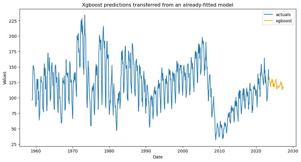
f_new = pipeline_new.fit_predict(f_new,transfer_from=f) # even though it says fit, no model actually gets fit in the pipeline

f_new.plot()
plt.title('Xgboost predictions transferred from an already-fitted model')
plt.show()