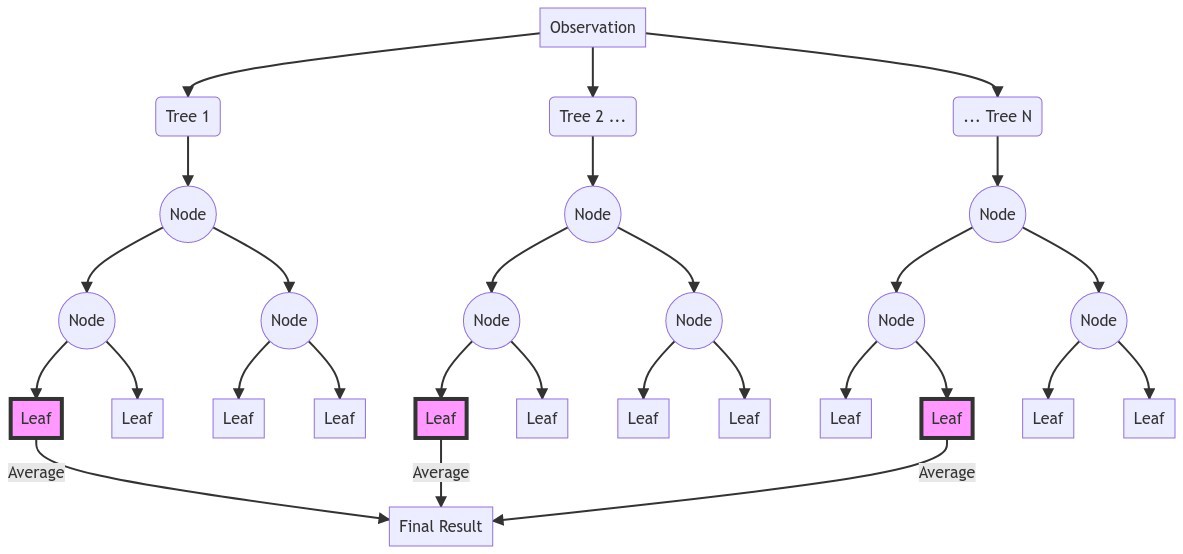
Scikit-Learn Models
This notebook showcases the scalecast wrapper around scikit-learn models.
[1]:
import pandas as pd
import numpy as np
import pandas_datareader as pdr
import matplotlib
import matplotlib.pyplot as plt
import seaborn as sns
from dateutil.relativedelta import relativedelta
from scalecast.Forecaster import Forecaster
from scalecast import GridGenerator
from scalecast.auxmodels import mlp_stack
from tqdm.notebook import tqdm
from sklearn.ensemble import BaggingRegressor
from sklearn.ensemble import StackingRegressor
from sklearn.neural_network import MLPRegressor

pd.set_option('max_colwidth',500)
pd.set_option('display.max_rows',500)
[2]:
def plot_test_export_summaries(f):
    """ exports the relevant statisitcal information and displays a plot of the test-set results for the last model run
    """
    f.plot_test_set(models=f.estimator,ci=True)
    plt.title(f'{f.estimator} test-set results',size=16)
    plt.show()
    return f.export('model_summaries',determine_best_by='TestSetMAPE')[
        [
            'ModelNickname',
            'HyperParams',
            'TestSetMAPE',
            'TestSetR2',
            'InSampleMAPE',
            'InSampleR2'
        ]
    ]
We will bring in the default grids from scalecast and tune some of our models this way. For others, we will create our own grids.
[3]:
GridGenerator.get_example_grids()
[4]:
data = pd.read_csv('daily-website-visitors.csv')
data.head()
[4]:
| Row | Day | Day.Of.Week | Date | Page.Loads | Unique.Visits | First.Time.Visits | Returning.Visits | |
|---|---|---|---|---|---|---|---|---|
| 0 | 1 | Sunday | 1 | 9/14/2014 | 2,146 | 1,582 | 1430 | 152 |
| 1 | 2 | Monday | 2 | 9/15/2014 | 3,621 | 2,528 | 2297 | 231 |
| 2 | 3 | Tuesday | 3 | 9/16/2014 | 3,698 | 2,630 | 2352 | 278 |
| 3 | 4 | Wednesday | 4 | 9/17/2014 | 3,667 | 2,614 | 2327 | 287 |
| 4 | 5 | Thursday | 5 | 9/18/2014 | 3,316 | 2,366 | 2130 | 236 |
[5]:
data.shape
[5]:
(2167, 8)
[6]:
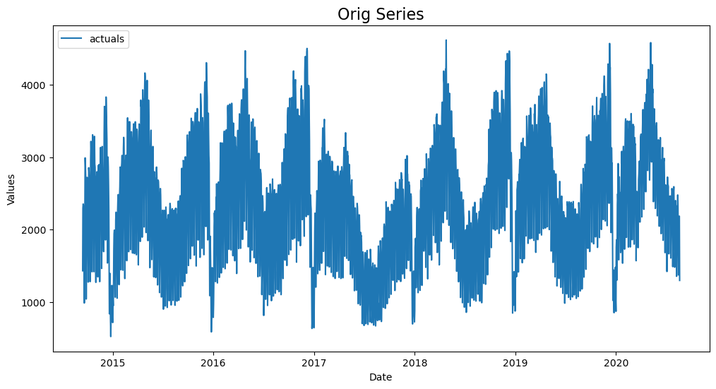
f=Forecaster(y=data['First.Time.Visits'],current_dates=data['Date'])
f.plot()
plt.title('Orig Series',size=16)
plt.show()
Not all models we will showcase come standard in scalecast, but we can easily add them by using the code below:
[7]:
f.add_sklearn_estimator(BaggingRegressor,'bagging')
f.add_sklearn_estimator(StackingRegressor,'stacking')
For more EDA on this dataset, see the prophet example: https://scalecast-examples.readthedocs.io/en/latest/prophet/prophet.html#EDA
Prepare Forecast
60-day forecast horizon
20% test split
Turn confidence intervals on
Add time series regressors:
7 autoregressive terms
4 seasonal autoregressive terms spaced 7-periods apart
month, quarter, week, and day of year with a fournier transformation
dayofweek, leap year, and week as dummy variables
year
[8]:
fcst_length = 60
f.generate_future_dates(fcst_length)
f.set_test_length(.2)
f.eval_cis() # tell the object to build confidence intervals for all models
f.add_ar_terms(7)
f.add_AR_terms((4,7))
f.add_seasonal_regressors('month','quarter','week','dayofyear',raw=False,sincos=True)
f.add_seasonal_regressors('dayofweek','is_leap_year','week',raw=False,dummy=True,drop_first=True)
f.add_seasonal_regressors('year')
f
[8]:
Forecaster(
    DateStartActuals=2014-09-14T00:00:00.000000000
    DateEndActuals=2020-08-19T00:00:00.000000000
    Freq=D
    N_actuals=2167
    ForecastLength=60
    Xvars=['AR1', 'AR2', 'AR3', 'AR4', 'AR5', 'AR6', 'AR7', 'AR14', 'AR21', 'AR28', 'monthsin', 'monthcos', 'quartersin', 'quartercos', 'weeksin', 'weekcos', 'dayofyearsin', 'dayofyearcos', 'dayofweek_1', 'dayofweek_2', 'dayofweek_3', 'dayofweek_4', 'dayofweek_5', 'dayofweek_6', 'is_leap_year_True', 'week_10', 'week_11', 'week_12', 'week_13', 'week_14', 'week_15', 'week_16', 'week_17', 'week_18', 'week_19', 'week_2', 'week_20', 'week_21', 'week_22', 'week_23', 'week_24', 'week_25', 'week_26', 'week_27', 'week_28', 'week_29', 'week_3', 'week_30', 'week_31', 'week_32', 'week_33', 'week_34', 'week_35', 'week_36', 'week_37', 'week_38', 'week_39', 'week_4', 'week_40', 'week_41', 'week_42', 'week_43', 'week_44', 'week_45', 'week_46', 'week_47', 'week_48', 'week_49', 'week_5', 'week_50', 'week_51', 'week_52', 'week_53', 'week_6', 'week_7', 'week_8', 'week_9', 'year']
    TestLength=433
    ValidationMetric=rmse
    ForecastsEvaluated=[]
    CILevel=0.95
    CurrentEstimator=mlr
    GridsFile=Grids
)
MLR
use default parameters (which means all input vars are scaled with a minmax scaler by default for all sklearn models)
[9]:
f.set_estimator('mlr')
f.manual_forecast()
[10]:
plot_test_export_summaries(f)

[10]:
| ModelNickname | HyperParams | TestSetMAPE | TestSetR2 | InSampleMAPE | InSampleR2 | |
|---|---|---|---|---|---|---|
| 0 | mlr | {} | 0.14485 | 0.733553 | 0.064183 | 0.953482 |
Lasso
tune alpha with 100 choices using 3-fold cross validation
[11]:
f.set_estimator('lasso')
lasso_grid = {'alpha':np.linspace(0,2,100)}
f.ingest_grid(lasso_grid)
f.cross_validate(k=3)
f.auto_forecast()
[12]:
plot_test_export_summaries(f)
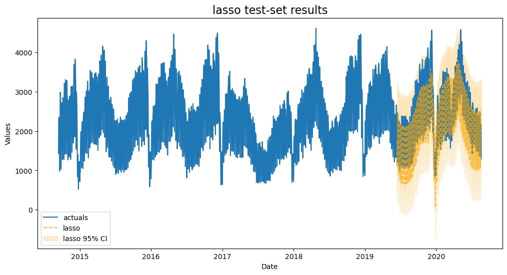
[12]:
| ModelNickname | HyperParams | TestSetMAPE | TestSetR2 | InSampleMAPE | InSampleR2 | |
|---|---|---|---|---|---|---|
| 0 | lasso | {'alpha': 0.32323232323232326} | 0.139526 | 0.744279 | 0.065458 | 0.952205 |
| 1 | mlr | {} | 0.144850 | 0.733553 | 0.064183 | 0.953482 |
Ridge
tune alpha with the same grid used for lasso
[13]:
f.set_estimator('ridge')
f.ingest_grid(lasso_grid)
f.cross_validate(k=3)
f.auto_forecast()
[14]:
plot_test_export_summaries(f)
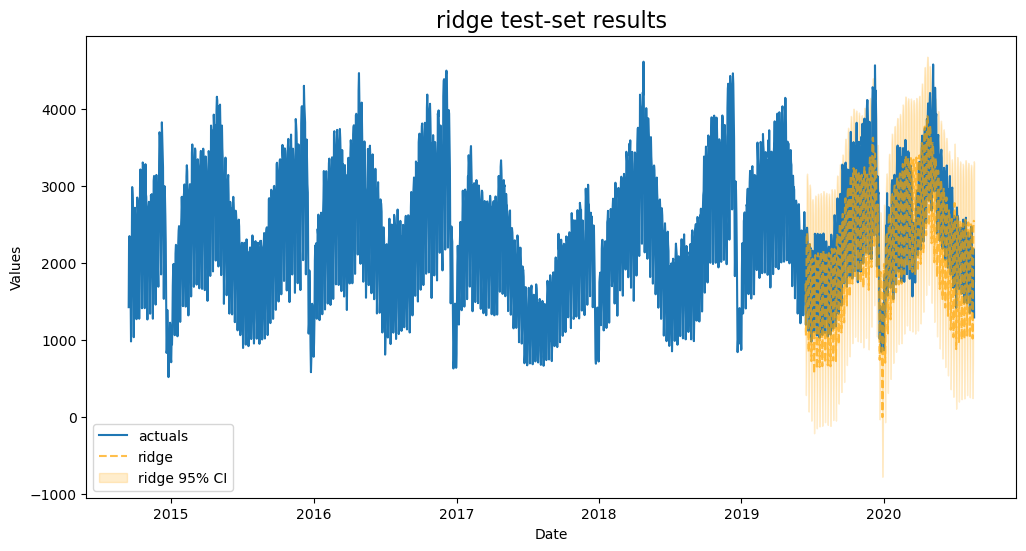
[14]:
| ModelNickname | HyperParams | TestSetMAPE | TestSetR2 | InSampleMAPE | InSampleR2 | |
|---|---|---|---|---|---|---|
| 0 | lasso | {'alpha': 0.32323232323232326} | 0.139526 | 0.744279 | 0.065458 | 0.952205 |
| 1 | ridge | {'alpha': 0.6060606060606061} | 0.140560 | 0.743738 | 0.064592 | 0.952812 |
| 2 | mlr | {} | 0.144850 | 0.733553 | 0.064183 | 0.953482 |
Elasticnet
this model mixes L1 and L2 regularization parameters
its default grid is pretty good for finding the optimal alpha value and l1 ratio
[15]:
f.set_estimator('elasticnet')
f.cross_validate(k=3)
f.auto_forecast()
[16]:
plot_test_export_summaries(f)
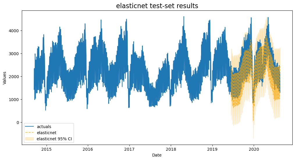
[16]:
| ModelNickname | HyperParams | TestSetMAPE | TestSetR2 | InSampleMAPE | InSampleR2 | |
|---|---|---|---|---|---|---|
| 0 | lasso | {'alpha': 0.32323232323232326} | 0.139526 | 0.744279 | 0.065458 | 0.952205 |
| 1 | ridge | {'alpha': 0.6060606060606061} | 0.140560 | 0.743738 | 0.064592 | 0.952812 |
| 2 | elasticnet | {'alpha': 2.0, 'l1_ratio': 1, 'normalizer': 'scale'} | 0.141774 | 0.733125 | 0.065364 | 0.952024 |
| 3 | mlr | {} | 0.144850 | 0.733553 | 0.064183 | 0.953482 |
RF
create a grid to tune Random Forest with more options than what is available in the default grids
[17]:
f.set_estimator('rf')
rf_grid = {
    'max_depth':[2,3,4,5],
    'n_estimators':[100,200,500],
    'max_features':['auto','sqrt','log2'],
    'max_samples':[.75,.9,1],
}
f.ingest_grid(rf_grid)
f.cross_validate(k=3)
f.auto_forecast()
[18]:
plot_test_export_summaries(f)
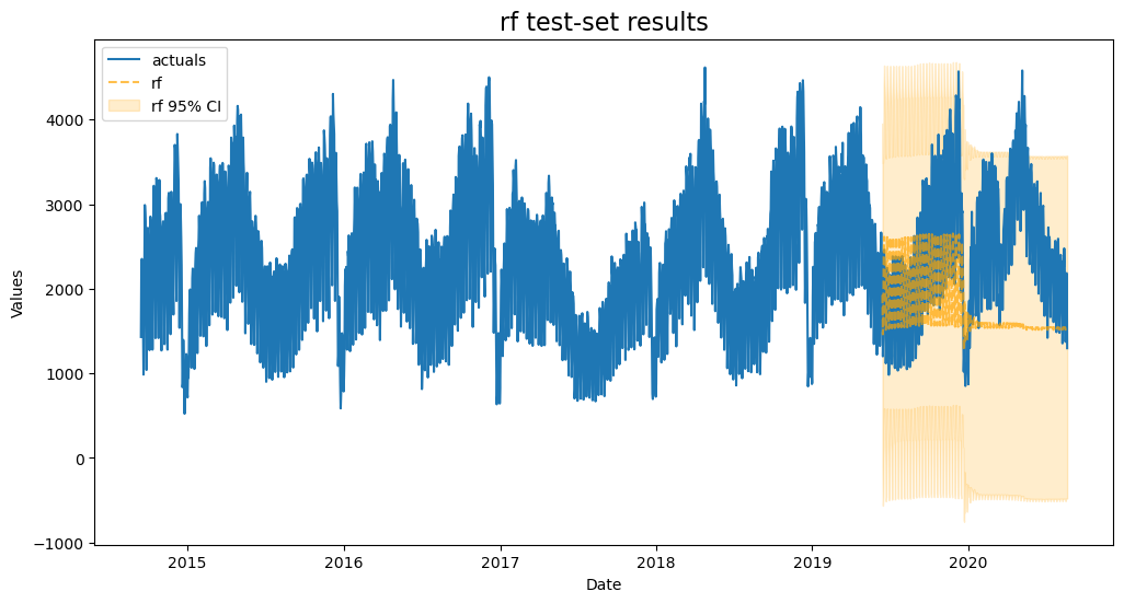
[18]:
| ModelNickname | HyperParams | TestSetMAPE | TestSetR2 | InSampleMAPE | InSampleR2 | |
|---|---|---|---|---|---|---|
| 0 | lasso | {'alpha': 0.32323232323232326} | 0.139526 | 0.744279 | 0.065458 | 0.952205 |
| 1 | ridge | {'alpha': 0.6060606060606061} | 0.140560 | 0.743738 | 0.064592 | 0.952812 |
| 2 | mlr | {} | 0.144850 | 0.733553 | 0.064183 | 0.953482 |
| 3 | elasticnet | {'alpha': 2.0, 'l1_ratio': 0, 'normalizer': None} | 0.259322 | 0.152033 | 0.092402 | 0.904719 |
| 4 | rf | {'max_depth': 5, 'n_estimators': 200, 'max_features': 'auto', 'max_samples': 0.75} | 0.318096 | -0.916329 | 0.083374 | 0.918095 |
So far, both using a visual inspection and examing its test-set performance, Random Forest does worse than all others.
XGBoost
Build a grid to tune XGBoost
[19]:
f.set_estimator('xgboost')
xgboost_grid = {
     'n_estimators':[150,200,250],
     'scale_pos_weight':[5,10],
     'learning_rate':[0.1,0.2],
     'gamma':[0,3,5],
     'subsample':[0.8,0.9]
}
f.ingest_grid(xgboost_grid)
f.cross_validate(k=3)
f.auto_forecast()
[20]:
plot_test_export_summaries(f)
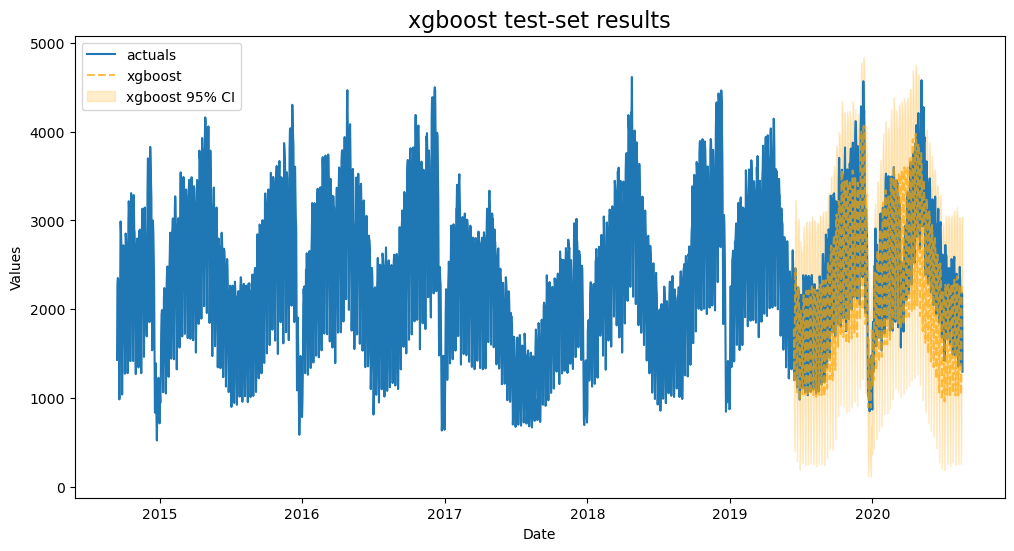
[20]:
| ModelNickname | HyperParams | TestSetMAPE | TestSetR2 | InSampleMAPE | InSampleR2 | |
|---|---|---|---|---|---|---|
| 0 | xgboost | {'n_estimators': 150, 'scale_pos_weight': 5, 'learning_rate': 0.1, 'gamma': 5, 'subsample': 0.9} | 0.115551 | 0.769377 | 0.018676 | 0.995667 |
| 1 | lasso | {'alpha': 0.32323232323232326} | 0.139526 | 0.744279 | 0.065458 | 0.952205 |
| 2 | ridge | {'alpha': 0.6060606060606061} | 0.140560 | 0.743738 | 0.064592 | 0.952812 |
| 3 | mlr | {} | 0.144850 | 0.733553 | 0.064183 | 0.953482 |
| 4 | elasticnet | {'alpha': 2.0, 'l1_ratio': 0, 'normalizer': None} | 0.259322 | 0.152033 | 0.092402 | 0.904719 |
| 5 | rf | {'max_depth': 5, 'n_estimators': 200, 'max_features': 'auto', 'max_samples': 0.75} | 0.318096 | -0.916329 | 0.083374 | 0.918095 |
This is our best model so far using the test MAPE as the metric to determine that by. It appears to be also be highly overfit.
LightGBM
Build a grid to tune LightGBM
[21]:
f.set_estimator('lightgbm')
lightgbm_grid = {
    'n_estimators':[150,200,250],
    'boosting_type':['gbdt','dart','goss'],
    'max_depth':[1,2,3],
    'learning_rate':[0.001,0.01,0.1],
    'reg_alpha':np.linspace(0,1,5),
    'reg_lambda':np.linspace(0,1,5),
    'num_leaves':np.arange(5,50,5),
}
f.ingest_grid(lightgbm_grid)
f.limit_grid_size(100,random_seed=2)
f.cross_validate(k=3)
f.auto_forecast()
[22]:
plot_test_export_summaries(f)
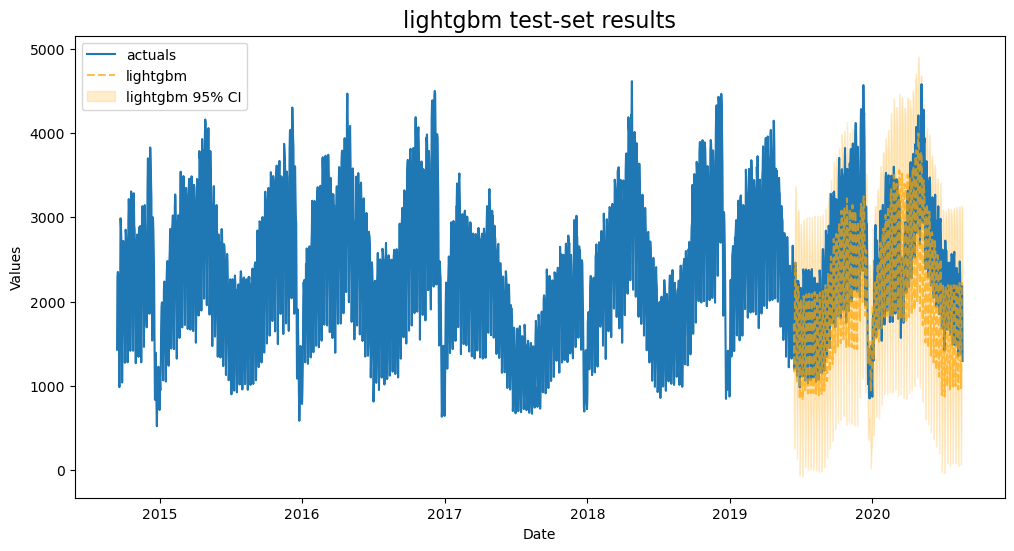
[22]:
| ModelNickname | HyperParams | TestSetMAPE | TestSetR2 | InSampleMAPE | InSampleR2 | |
|---|---|---|---|---|---|---|
| 0 | xgboost | {'n_estimators': 150, 'scale_pos_weight': 5, 'learning_rate': 0.1, 'gamma': 5, 'subsample': 0.9} | 0.115551 | 0.769377 | 0.018676 | 0.995667 |
| 1 | lasso | {'alpha': 0.32323232323232326} | 0.139526 | 0.744279 | 0.065458 | 0.952205 |
| 2 | ridge | {'alpha': 0.6060606060606061} | 0.140560 | 0.743738 | 0.064592 | 0.952812 |
| 3 | mlr | {} | 0.144850 | 0.733553 | 0.064183 | 0.953482 |
| 4 | lightgbm | {'n_estimators': 200, 'boosting_type': 'goss', 'max_depth': 3, 'learning_rate': 0.1, 'reg_alpha': 0.25, 'reg_lambda': 1.0, 'num_leaves': 35} | 0.166747 | 0.592318 | 0.050726 | 0.970159 |
| 5 | elasticnet | {'alpha': 2.0, 'l1_ratio': 0, 'normalizer': None} | 0.259322 | 0.152033 | 0.092402 | 0.904719 |
| 6 | rf | {'max_depth': 5, 'n_estimators': 200, 'max_features': 'auto', 'max_samples': 0.75} | 0.318096 | -0.916329 | 0.083374 | 0.918095 |
SGD
Use the default Stochastic Gradient Descent grid
[23]:
f.set_estimator('sgd')
f.cross_validate(k=3)
f.auto_forecast()
Finished loading model, total used 200 iterations
Finished loading model, total used 200 iterations
Finished loading model, total used 200 iterations
Finished loading model, total used 200 iterations
Finished loading model, total used 200 iterations
[24]:
plot_test_export_summaries(f)
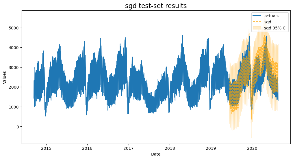
[24]:
| ModelNickname | HyperParams | TestSetMAPE | TestSetR2 | InSampleMAPE | InSampleR2 | |
|---|---|---|---|---|---|---|
| 0 | xgboost | {'n_estimators': 150, 'scale_pos_weight': 5, 'learning_rate': 0.1, 'gamma': 5, 'subsample': 0.9} | 0.115551 | 0.769377 | 0.018676 | 0.995667 |
| 1 | lasso | {'alpha': 0.32323232323232326} | 0.139526 | 0.744279 | 0.065458 | 0.952205 |
| 2 | ridge | {'alpha': 0.6060606060606061} | 0.140560 | 0.743738 | 0.064592 | 0.952812 |
| 3 | mlr | {} | 0.144850 | 0.733553 | 0.064183 | 0.953482 |
| 4 | sgd | {'penalty': 'elasticnet', 'l1_ratio': 1, 'learning_rate': 'constant'} | 0.166129 | 0.609554 | 0.065153 | 0.951795 |
| 5 | lightgbm | {'n_estimators': 200, 'boosting_type': 'goss', 'max_depth': 3, 'learning_rate': 0.1, 'reg_alpha': 0.25, 'reg_lambda': 1.0, 'num_leaves': 35} | 0.166747 | 0.592318 | 0.050726 | 0.970159 |
| 6 | elasticnet | {'alpha': 2.0, 'l1_ratio': 0, 'normalizer': None} | 0.259322 | 0.152033 | 0.092402 | 0.904719 |
| 7 | rf | {'max_depth': 5, 'n_estimators': 200, 'max_features': 'auto', 'max_samples': 0.75} | 0.318096 | -0.916329 | 0.083374 | 0.918095 |
KNN
Use the default K-nearest Neighbors grid
[25]:
f.set_estimator('knn')
f.cross_validate(k=3)
f.auto_forecast()
Finished loading model, total used 200 iterations
Finished loading model, total used 200 iterations
Finished loading model, total used 200 iterations
Finished loading model, total used 200 iterations
Finished loading model, total used 200 iterations
[26]:
plot_test_export_summaries(f)
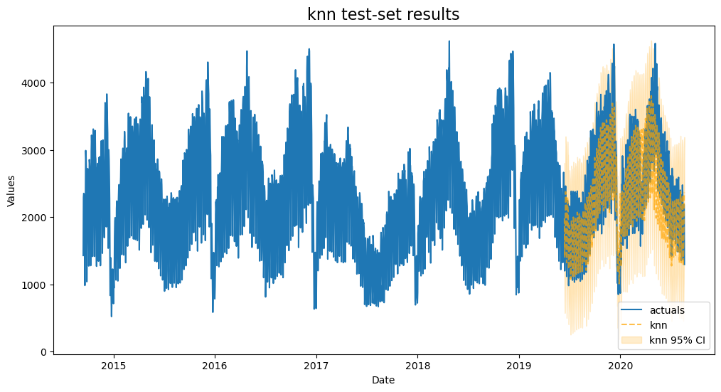
[26]:
| ModelNickname | HyperParams | TestSetMAPE | TestSetR2 | InSampleMAPE | InSampleR2 | |
|---|---|---|---|---|---|---|
| 0 | xgboost | {'n_estimators': 150, 'scale_pos_weight': 5, 'learning_rate': 0.1, 'gamma': 5, 'subsample': 0.9} | 0.115551 | 0.769377 | 0.018676 | 0.995667 |
| 1 | knn | {'n_neighbors': 20, 'weights': 'uniform'} | 0.130121 | 0.713268 | 0.117198 | 0.873220 |
| 2 | lasso | {'alpha': 0.32323232323232326} | 0.139526 | 0.744279 | 0.065458 | 0.952205 |
| 3 | ridge | {'alpha': 0.6060606060606061} | 0.140560 | 0.743738 | 0.064592 | 0.952812 |
| 4 | mlr | {} | 0.144850 | 0.733553 | 0.064183 | 0.953482 |
| 5 | sgd | {'penalty': 'elasticnet', 'l1_ratio': 1, 'learning_rate': 'constant'} | 0.166129 | 0.609554 | 0.065153 | 0.951795 |
| 6 | lightgbm | {'n_estimators': 200, 'boosting_type': 'goss', 'max_depth': 3, 'learning_rate': 0.1, 'reg_alpha': 0.25, 'reg_lambda': 1.0, 'num_leaves': 35} | 0.166747 | 0.592318 | 0.050726 | 0.970159 |
| 7 | elasticnet | {'alpha': 2.0, 'l1_ratio': 0, 'normalizer': None} | 0.259322 | 0.152033 | 0.092402 | 0.904719 |
| 8 | rf | {'max_depth': 5, 'n_estimators': 200, 'max_features': 'auto', 'max_samples': 0.75} | 0.318096 | -0.916329 | 0.083374 | 0.918095 |
KNN is our most overfit model so far, but it fits the test-set pretty well.
BaggingRegressor
Like Random Forest is a bagging ensemble model using decision trees, we can use a bagging estimator that uses a three-layered mulit-level perceptron to see if the added complexity improves where the Random Forest couldn’t
[28]:
f.set_estimator('bagging')
f.manual_forecast(
    base_estimator = MLPRegressor(
        hidden_layer_sizes=(100,100,100)
        ,solver='lbfgs'
    ),
    max_samples = 0.9,
    max_features = 0.5,
)
Finished loading model, total used 200 iterations
[29]:
plot_test_export_summaries(f)
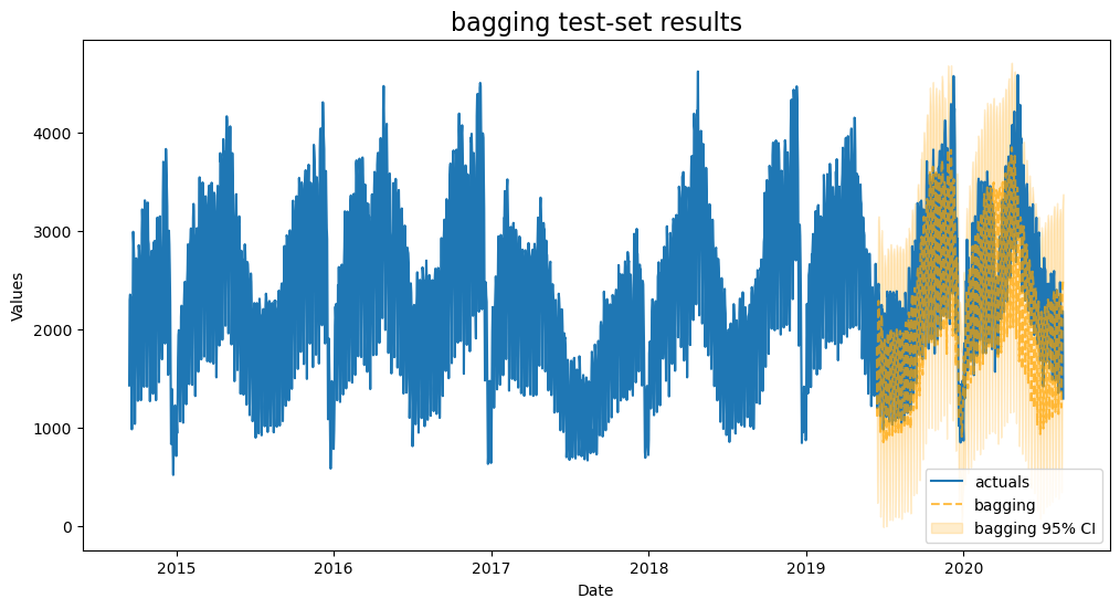
[29]:
| ModelNickname | HyperParams | TestSetMAPE | TestSetR2 | InSampleMAPE | InSampleR2 | |
|---|---|---|---|---|---|---|
| 0 | xgboost | {'n_estimators': 150, 'scale_pos_weight': 5, 'learning_rate': 0.1, 'gamma': 5, 'subsample': 0.9} | 0.115551 | 0.769377 | 0.018676 | 0.995667 |
| 1 | knn | {'n_neighbors': 20, 'weights': 'uniform'} | 0.130121 | 0.713268 | 0.117198 | 0.873220 |
| 2 | bagging | {'base_estimator': MLPRegressor(hidden_layer_sizes=(100, 100, 100), solver='lbfgs'), 'max_samples': 0.9, 'max_features': 0.5} | 0.130137 | 0.714881 | 0.050964 | 0.967984 |
| 3 | lasso | {'alpha': 0.32323232323232326} | 0.139526 | 0.744279 | 0.065458 | 0.952205 |
| 4 | ridge | {'alpha': 0.6060606060606061} | 0.140560 | 0.743738 | 0.064592 | 0.952812 |
| 5 | mlr | {} | 0.144850 | 0.733553 | 0.064183 | 0.953482 |
| 6 | sgd | {'penalty': 'elasticnet', 'l1_ratio': 1, 'learning_rate': 'constant'} | 0.166129 | 0.609554 | 0.065153 | 0.951795 |
| 7 | lightgbm | {'n_estimators': 200, 'boosting_type': 'goss', 'max_depth': 3, 'learning_rate': 0.1, 'reg_alpha': 0.25, 'reg_lambda': 1.0, 'num_leaves': 35} | 0.166747 | 0.592318 | 0.050726 | 0.970159 |
| 8 | elasticnet | {'alpha': 2.0, 'l1_ratio': 0, 'normalizer': None} | 0.259322 | 0.152033 | 0.092402 | 0.904719 |
| 9 | rf | {'max_depth': 5, 'n_estimators': 200, 'max_features': 'auto', 'max_samples': 0.75} | 0.318096 | -0.916329 | 0.083374 | 0.918095 |
This is the best-performing model yet, with less overfitting than XGBoost and KNN.
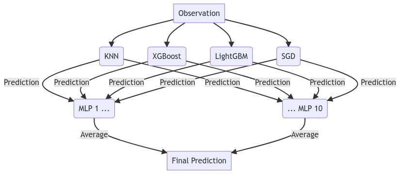
StackingRegressor
This model will use the predictions of other models as inputs to a “final estimator”. It’s added complexity can mean better performance, although not always.
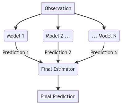
The model that we employ uses the bagged MLP regressor from the previous section as its final estimator, and the tuned knn, xgboost, lightgbm, and sgd models as its inputs.
[30]:
f.plot_fitted()
plt.title('all models fitted vals',size=16)
plt.show()
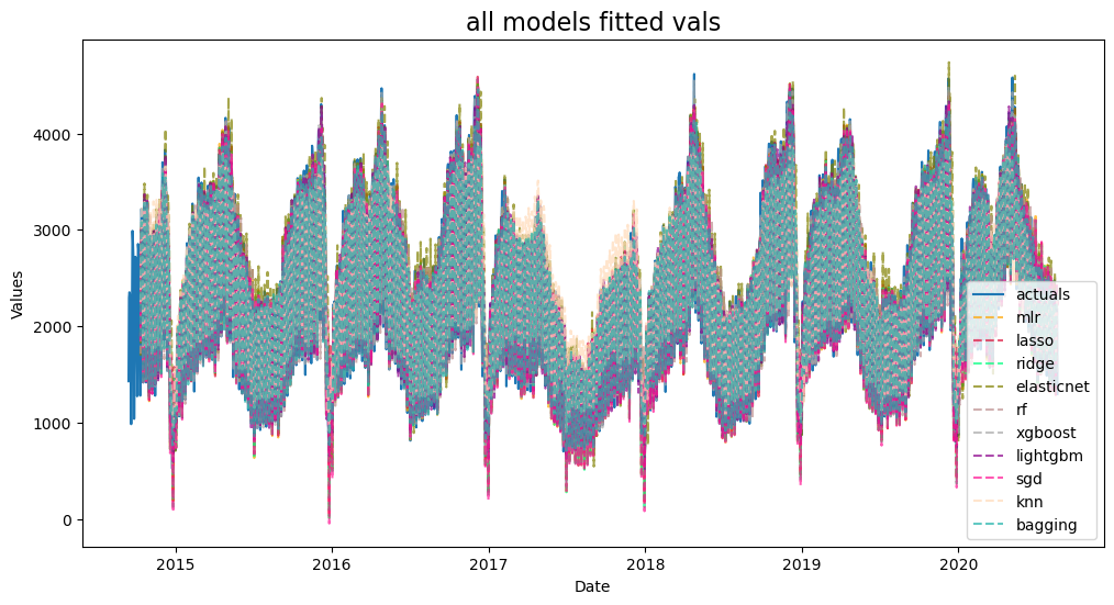
Sometimes seeing the fitted values can give a good idea of which models to stack, as you want models that can predict both the highs and lows of the series. However, this graph didn’t tell us much.
We use four of our best performing models to create the model inputs. We use a bagging estimator as the final model.
[31]:
f.set_estimator('stacking')
results = f.export('model_summaries')
estimators = [
'knn',
'xgboost',
'lightgbm',
'sgd',
]
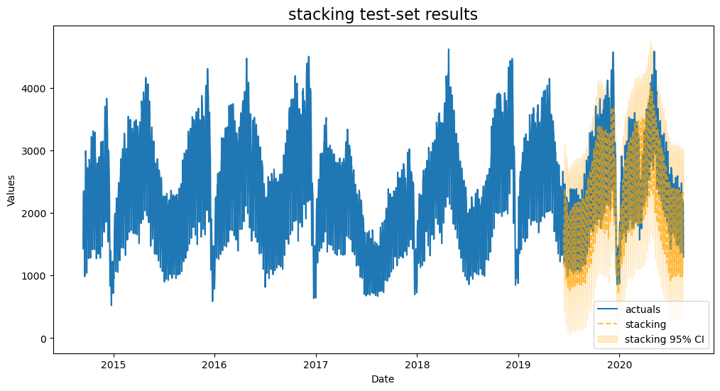
mlp_stack(f,estimators,call_me='stacking')
Finished loading model, total used 200 iterations
[32]:
plot_test_export_summaries(f)
[32]:
| ModelNickname | HyperParams | TestSetMAPE | TestSetR2 | InSampleMAPE | InSampleR2 | |
|---|---|---|---|---|---|---|
| 0 | xgboost | {'n_estimators': 150, 'scale_pos_weight': 5, 'learning_rate': 0.1, 'gamma': 5, 'subsample': 0.9} | 0.115551 | 0.769377 | 0.018676 | 0.995667 |
| 1 | stacking | {'estimators': [('knn', KNeighborsRegressor(n_neighbors=20)), ('xgboost', XGBRegressor(base_score=None, booster=None, callbacks=None, colsample_bylevel=None, colsample_bynode=None, colsample_bytree=None, early_stopping_rounds=None, enable_categorical=False, eval_metric=None, feature_types=None, gamma=5, gpu_id=None, grow_policy=None, importance_type=None, interaction_constraints=None, learning_rate=0.1, max_bin=None, ... | 0.122353 | 0.784423 | 0.040845 | 0.979992 |
| 2 | knn | {'n_neighbors': 20, 'weights': 'uniform'} | 0.130121 | 0.713268 | 0.117198 | 0.873220 |
| 3 | bagging | {'base_estimator': MLPRegressor(hidden_layer_sizes=(100, 100, 100), solver='lbfgs'), 'max_samples': 0.9, 'max_features': 0.5} | 0.130137 | 0.714881 | 0.050964 | 0.967984 |
| 4 | lasso | {'alpha': 0.32323232323232326} | 0.139526 | 0.744279 | 0.065458 | 0.952205 |
| 5 | ridge | {'alpha': 0.6060606060606061} | 0.140560 | 0.743738 | 0.064592 | 0.952812 |
| 6 | mlr | {} | 0.144850 | 0.733553 | 0.064183 | 0.953482 |
| 7 | sgd | {'penalty': 'elasticnet', 'l1_ratio': 1, 'learning_rate': 'constant'} | 0.166129 | 0.609554 | 0.065153 | 0.951795 |
| 8 | lightgbm | {'n_estimators': 200, 'boosting_type': 'goss', 'max_depth': 3, 'learning_rate': 0.1, 'reg_alpha': 0.25, 'reg_lambda': 1.0, 'num_leaves': 35} | 0.166747 | 0.592318 | 0.050726 | 0.970159 |
| 9 | elasticnet | {'alpha': 2.0, 'l1_ratio': 0, 'normalizer': None} | 0.259322 | 0.152033 | 0.092402 | 0.904719 |
| 10 | rf | {'max_depth': 5, 'n_estimators': 200, 'max_features': 'auto', 'max_samples': 0.75} | 0.318096 | -0.916329 | 0.083374 | 0.918095 |
This is our best model with lower amounts of overfitting than some of our other models. We will choose it to make our final forecasts with.
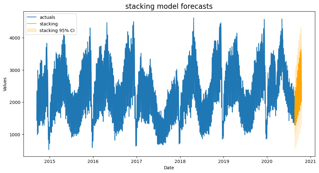
Plot Forecast
[33]:
f.plot('stacking',ci=True)
plt.title('stacking model forecasts',size=16)
plt.show()
[ ]: