Confidence Intervals
This notebook overviews scalecast intervals, which are scored with Mean Scaled Interval Score (MSIS). Lower scores are better. This notebook requires scalecast>=0.18.0.
Scalecast uses a naive conformal interval, created from holding out a test-set of data and setting interval ranges from the percentiles of the test-set residuals. This simple approach allows every estimator type to get the same kind of interval. As we will see by scoring the intervals and comparing them to ARIMA intervals from statsmodels, the results are good.
To evaluate the intervals, we leave out a section of each series to score out-of-sample. This is usually not necessary for scalecast, as all models are tested automatically, but the confidence intervals can overfit on any test set stored in the Forecaster or MVForecaster object due to leakage that occurs when constructing these intervals. Scalecast intervals are compared to ARIMA intervals on the same series in the last section of this notebook and the scalecast intervals, on the whole,
perform better. The series used in this example are ordered from easiest-to-hardest to forecast.
Easy Distribution-Free Conformal Intervals for Time Series
[1]:
import pandas as pd
import numpy as np
from scalecast.Forecaster import Forecaster
from scalecast import GridGenerator
from scalecast.util import metrics
from scalecast.notebook import tune_test_forecast
from scalecast.SeriesTransformer import SeriesTransformer
import matplotlib.pyplot as plt
import seaborn as sns
import time
from tqdm.notebook import tqdm
[2]:
import warnings
warnings.simplefilter(action='ignore', category=DeprecationWarning)
[3]:
models = (
    'mlr',
    'elasticnet',
    'ridge',
    'knn',
    'xgboost',
    'lightgbm',
    'gbt',
) # these are all scikit-learn models or APIs
# this will be used later to fill in results
results_template = pd.DataFrame(index=models)
[4]:
def score_cis(results, fcsts, ci_name, actuals, obs, val_len, models=models, m_=1):
    for m in models:
        results.loc[m,ci_name] = metrics.msis(
            a = actuals,
            uf = fcsts[m+'_upperci'],
            lf = fcsts[m+'_lowerci'],
            obs = obs,
            m = m_,
        )
    return results
[5]:
GridGenerator.get_example_grids()
Daily Website Visitors
Link to data: https://www.kaggle.com/datasets/bobnau/daily-website-visitors
We will use a length of 180 observations (about half a year) both to tune and test the models
We want to optimize the forecasts and confidence intervals for a 60-day forecast horizon
[6]:
val_len = 180
fcst_len = 60
[7]:
data = pd.read_csv('daily-website-visitors.csv',parse_dates=['Date']).set_index('Date')
data.head()
[7]:
| Row | Day | Day.Of.Week | Page.Loads | Unique.Visits | First.Time.Visits | Returning.Visits | |
|---|---|---|---|---|---|---|---|
| Date | |||||||
| 2014-09-14 | 1 | Sunday | 1 | 2,146 | 1,582 | 1430 | 152 |
| 2014-09-15 | 2 | Monday | 2 | 3,621 | 2,528 | 2297 | 231 |
| 2014-09-16 | 3 | Tuesday | 3 | 3,698 | 2,630 | 2352 | 278 |
| 2014-09-17 | 4 | Wednesday | 4 | 3,667 | 2,614 | 2327 | 287 |
| 2014-09-18 | 5 | Thursday | 5 | 3,316 | 2,366 | 2130 | 236 |
[8]:
visits_sep = data['First.Time.Visits'].iloc[-fcst_len:]
visits = data['First.Time.Visits'].iloc[:-fcst_len]
[9]:
f=Forecaster(
    y=visits,
    current_dates=visits.index,
    future_dates=fcst_len,
    test_length = val_len,
    validation_length = val_len, # for hyperparameter tuning
    cis = True, # set to True at initialization to always evaluate cis
)
f.auto_Xvar_select(
    estimator='elasticnet',
    alpha=.2,
    max_ar=100,
    monitor='ValidationMetricValue',
)
f
[9]:
Forecaster(
    DateStartActuals=2014-09-14T00:00:00.000000000
    DateEndActuals=2020-06-20T00:00:00.000000000
    Freq=D
    N_actuals=2107
    ForecastLength=60
    Xvars=['t', 'AR1', 'AR2', 'AR3', 'AR4', 'AR5', 'AR6', 'AR7', 'AR8', 'AR9', 'AR10', 'AR11', 'AR12', 'AR13', 'AR14', 'AR15', 'AR16', 'AR17', 'AR18', 'AR19', 'AR20', 'AR21', 'AR22', 'AR23', 'AR24', 'AR25', 'AR26', 'AR27', 'AR28', 'AR29', 'AR30', 'AR31', 'AR32', 'AR33', 'AR34', 'AR35', 'AR36', 'AR37', 'AR38', 'AR39', 'AR40', 'AR41', 'AR42', 'AR43', 'AR44', 'AR45', 'AR46', 'AR47', 'AR48', 'AR49', 'AR50', 'AR51', 'AR52', 'AR53', 'AR54', 'AR55', 'AR56', 'AR57', 'AR58', 'AR59', 'AR60', 'AR61', 'AR62', 'AR63', 'AR64', 'AR65', 'AR66', 'AR67', 'AR68', 'AR69', 'AR70', 'AR71', 'AR72', 'AR73', 'AR74', 'AR75', 'AR76', 'AR77', 'AR78', 'AR79', 'AR80', 'AR81', 'AR82', 'AR83', 'AR84', 'AR85', 'AR86', 'AR87', 'AR88', 'AR89', 'AR90', 'AR91', 'AR92', 'AR93', 'AR94', 'AR95', 'AR96', 'AR97', 'AR98', 'AR99', 'AR100']
    TestLength=180
    ValidationMetric=rmse
    ForecastsEvaluated=[]
    CILevel=0.95
    CurrentEstimator=mlr
    GridsFile=Grids
)
[10]:
tune_test_forecast(
    f,
    models,
)
Finished loading model, total used 250 iterations
Finished loading model, total used 250 iterations
Finished loading model, total used 250 iterations
[11]:
ms = f.export('model_summaries',determine_best_by='TestSetRMSE')
ms[['ModelNickname','TestSetRMSE','InSampleRMSE']]
[11]:
| ModelNickname | TestSetRMSE | InSampleRMSE | |
|---|---|---|---|
| 0 | xgboost | 532.374846 | 14.496801 |
| 1 | lightgbm | 582.261645 | 112.543232 |
| 2 | knn | 788.704950 | 306.828988 |
| 3 | elasticnet | 794.649818 | 186.616620 |
| 4 | ridge | 798.711718 | 187.026325 |
| 5 | mlr | 803.931314 | 185.620629 |
| 6 | gbt | 1171.782785 | 147.478748 |
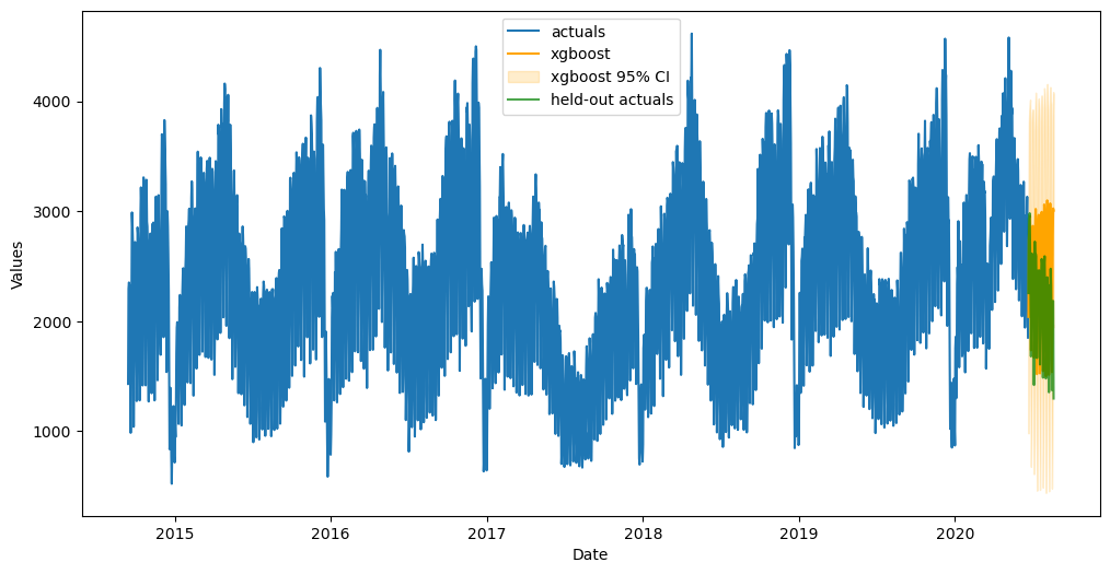
We will demonstrate how the confidence intervals change as they are re-evaluated using the best model according to the test RMSE.
Evaluate Interval
[12]:
fig, ax = plt.subplots(figsize=(12,6))
f.plot(ci=True,models='top_1',order_by='TestSetRMSE',ax=ax)
sns.lineplot(
    y = 'First.Time.Visits',
    x = 'Date',
    data = visits_sep.reset_index(),
    ax = ax,
    label = 'held-out actuals',
    color = 'green',
    alpha = 0.7,
)
plt.show()
[13]:
# export test-set preds and confidence intervals
fcsts1 = f.export("lvl_fcsts",cis=True)
fcsts1.head()
[13]:
| DATE | mlr | mlr_upperci | mlr_lowerci | elasticnet | elasticnet_upperci | elasticnet_lowerci | ridge | ridge_upperci | ridge_lowerci | ... | knn_lowerci | xgboost | xgboost_upperci | xgboost_lowerci | lightgbm | lightgbm_upperci | lightgbm_lowerci | gbt | gbt_upperci | gbt_lowerci | |
|---|---|---|---|---|---|---|---|---|---|---|---|---|---|---|---|---|---|---|---|---|---|
| 0 | 2020-06-21 | 2190.555279 | 3464.907755 | 916.202804 | 2194.962019 | 3452.970789 | 936.953250 | 2191.868075 | 3464.239858 | 919.496293 | ... | 812.176316 | 2039.648438 | 3098.496887 | 980.799988 | 2198.858468 | 3232.664729 | 1165.052207 | 2125.968510 | 4021.476092 | 230.460929 |
| 1 | 2020-06-22 | 2835.674158 | 4110.026633 | 1561.321683 | 2823.011263 | 4081.020033 | 1565.002493 | 2831.886812 | 4104.258594 | 1559.515029 | ... | 1612.281579 | 2743.368896 | 3802.217346 | 1684.520447 | 2820.575637 | 3854.381898 | 1786.769376 | 2729.050006 | 4624.557587 | 833.542425 |
| 2 | 2020-06-23 | 2975.510723 | 4249.863198 | 1701.158248 | 2944.846465 | 4202.855235 | 1686.837696 | 2972.183687 | 4244.555469 | 1699.811904 | ... | 1804.176316 | 2851.803711 | 3910.652161 | 1792.955261 | 2819.654176 | 3853.460437 | 1785.847915 | 2880.262061 | 4775.769642 | 984.754480 |
| 3 | 2020-06-24 | 3038.258157 | 4312.610632 | 1763.905681 | 3006.932564 | 4264.941333 | 1748.923794 | 3033.992818 | 4306.364600 | 1761.621035 | ... | 1673.860526 | 2905.132568 | 3963.981018 | 1846.284119 | 2824.992206 | 3858.798467 | 1791.185945 | 2930.293895 | 4825.801476 | 1034.786314 |
| 4 | 2020-06-25 | 3032.580568 | 4306.933043 | 1758.228093 | 3011.122478 | 4269.131247 | 1753.113708 | 3021.274091 | 4293.645873 | 1748.902309 | ... | 1475.386842 | 2955.912598 | 4014.761047 | 1897.064148 | 2961.588543 | 3995.394805 | 1927.782282 | 3029.007375 | 4924.514956 | 1133.499794 |
5 rows × 22 columns
The values in the below table are mean scaled interval scores for confidence intervals. Lower scores are better.
[14]:
results = score_cis(
    results_template.copy(),
    fcsts1,
    'Daily Visitors',
    visits_sep,
    visits,
    val_len = val_len,
)
results
[14]:
| Daily Visitors | |
|---|---|
| mlr | 5.632456 |
| elasticnet | 5.548336 |
| ridge | 5.622506 |
| knn | 5.639715 |
| xgboost | 5.597762 |
| lightgbm | 5.196714 |
| gbt | 8.319963 |
Housing Starts
Link to data: https://fred.stlouisfed.org/series/HOUSTNSA
We will use a length of 96 observations (8 years) both to tune and test the models
We want to optimize the forecasts and confidence intervals for a 24-month forecast horizon
[15]:
import pandas_datareader as pdr
[16]:
val_len = 96
fcst_len = 24
[17]:
housing = pdr.get_data_fred('HOUSTNSA',start='1900-01-01',end='2021-06-01')
housing.head()
[17]:
| HOUSTNSA | |
|---|---|
| DATE | |
| 1959-01-01 | 96.2 |
| 1959-02-01 | 99.0 |
| 1959-03-01 | 127.7 |
| 1959-04-01 | 150.8 |
| 1959-05-01 | 152.5 |
[18]:
starts_sep = housing.iloc[-fcst_len:,0]
starts = housing.iloc[:-fcst_len,0]
[19]:
f = Forecaster(
    y=starts,
    current_dates=starts.index,
    future_dates=fcst_len,
    test_length=val_len,
    validation_length=val_len,
    cis=True,
)
# difference the data for stationary modeling
transformer = SeriesTransformer(f)
f = transformer.DiffTransform(1)
# find best xvars to forecast with
f.auto_Xvar_select(
    estimator='elasticnet',
    alpha=.2,
    max_ar=100,
    monitor='ValidationMetricValue', # not test set
)
f
[19]:
Forecaster(
    DateStartActuals=1959-02-01T00:00:00.000000000
    DateEndActuals=2019-06-01T00:00:00.000000000
    Freq=MS
    N_actuals=725
    ForecastLength=24
    Xvars=['monthsin', 'monthcos', 'quartersin', 'quartercos', 'AR1', 'AR2', 'AR3', 'AR4', 'AR5', 'AR6', 'AR7', 'AR8', 'AR9', 'AR10', 'AR11', 'AR12', 'AR13', 'AR14', 'AR15', 'AR16', 'AR17', 'AR18', 'AR19', 'AR20', 'AR21', 'AR22', 'AR23', 'AR24', 'AR25', 'AR26', 'AR27', 'AR28', 'AR29', 'AR30', 'AR31', 'AR32', 'AR33', 'AR34', 'AR35', 'AR36', 'AR37', 'AR38', 'AR39', 'AR40', 'AR41', 'AR42', 'AR43', 'AR44', 'AR45', 'AR46', 'AR47', 'AR48', 'AR49', 'AR50', 'AR51', 'AR52', 'AR53', 'AR54', 'AR55', 'AR56', 'AR57', 'AR58', 'AR59', 'AR60', 'AR61', 'AR62', 'AR63', 'AR64', 'AR65', 'AR66', 'AR67', 'AR68', 'AR69', 'AR70', 'AR71', 'AR72', 'AR73', 'AR74', 'AR75', 'AR76', 'AR77', 'AR78', 'AR79', 'AR80', 'AR81', 'AR82', 'AR83', 'AR84', 'AR85', 'AR86', 'AR87', 'AR88', 'AR89', 'AR90', 'AR91', 'AR92', 'AR93', 'AR94', 'AR95', 'AR96', 'AR97', 'AR98', 'AR99', 'AR100']
    TestLength=96
    ValidationMetric=rmse
    ForecastsEvaluated=[]
    CILevel=0.95
    CurrentEstimator=mlr
    GridsFile=Grids
)
[20]:
tune_test_forecast(
    f,
    models,
    dynamic_testing = fcst_len,
)
Finished loading model, total used 150 iterations
Finished loading model, total used 150 iterations
Finished loading model, total used 150 iterations
[21]:
# rever the difftransform
f = transformer.DiffRevert(1)
[22]:
ms = f.export('model_summaries',determine_best_by='TestSetRMSE')
ms[['ModelNickname','TestSetRMSE','InSampleRMSE']]
[22]:
| ModelNickname | TestSetRMSE | InSampleRMSE | |
|---|---|---|---|
| 0 | xgboost | 21.402469 | 3.112793 |
| 1 | lightgbm | 23.160361 | 27.660879 |
| 2 | mlr | 30.059747 | 71.624715 |
| 3 | gbt | 38.185841 | 38.657789 |
| 4 | knn | 42.432505 | 146.502991 |
| 5 | ridge | 46.457215 | 55.969584 |
| 6 | elasticnet | 53.111686 | 38.237499 |
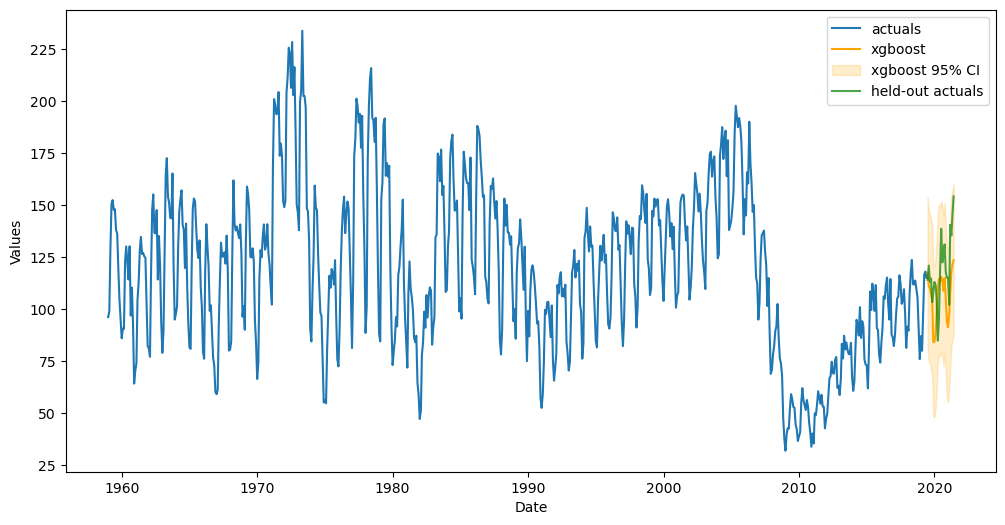
Evaluate Interval
[23]:
fig, ax = plt.subplots(figsize=(12,6))
f.plot(ci=True,models='top_1',order_by='TestSetRMSE',ax=ax)
sns.lineplot(
    y = 'HOUSTNSA',
    x = 'DATE',
    data = starts_sep.reset_index(),
    ax = ax,
    label = 'held-out actuals',
    color = 'green',
    alpha = 0.7,
)
plt.show()
[24]:
housing_fcsts1 = f.export("lvl_fcsts",cis=True)
housing_results = score_cis(
    results_template.copy(),
    housing_fcsts1,
    'Housing Starts',
    starts_sep,
    starts,
    val_len = val_len,
    m_ = 12, # monthly seasonality
)
housing_results
[24]:
| Housing Starts | |
|---|---|
| mlr | 5.661675 |
| elasticnet | 8.247183 |
| ridge | 7.432564 |
| knn | 6.552641 |
| xgboost | 3.930183 |
| lightgbm | 4.289493 |
| gbt | 5.884677 |
[25]:
results['Housing Starts'] = housing_results['Housing Starts']
results
[25]:
| Daily Visitors | Housing Starts | |
|---|---|---|
| mlr | 5.632456 | 5.661675 |
| elasticnet | 5.548336 | 8.247183 |
| ridge | 5.622506 | 7.432564 |
| knn | 5.639715 | 6.552641 |
| xgboost | 5.597762 | 3.930183 |
| lightgbm | 5.196714 | 4.289493 |
| gbt | 8.319963 | 5.884677 |
Avocado Sales
Link to data: https://www.kaggle.com/datasets/neuromusic/avocado-prices
We will use a length of 20 observations both to tune and test the models (95% CIs require at least 20 observations in the test set)
We want to optimize the forecasts and confidence intervals for a 20-week forecast horizon
[26]:
# change display settings
pd.options.display.float_format = '{:,.2f}'.format
[27]:
val_len = 20
fcst_len = 20
[28]:
avocados = pd.read_csv('avocado.csv',parse_dates = ['Date'])
volume = avocados.groupby('Date')['Total Volume'].sum()
[29]:
volume.reset_index().head()
[29]:
| Date | Total Volume | |
|---|---|---|
| 0 | 2015-01-04 | 84,674,337.20 |
| 1 | 2015-01-11 | 78,555,807.24 |
| 2 | 2015-01-18 | 78,388,784.08 |
| 3 | 2015-01-25 | 76,466,281.07 |
| 4 | 2015-02-01 | 119,453,235.25 |
[30]:
volume_sep = volume.iloc[-fcst_len:]
volume = volume.iloc[:-fcst_len]
[31]:
f = Forecaster(
    y = volume,
    current_dates = volume.index,
    future_dates = fcst_len,
    test_length = val_len,
    validation_length = val_len,
    cis = True,
)

# difference the data for stationary modeling
transformer = SeriesTransformer(f)
f = transformer.DiffTransform(1)
f = transformer.DiffTransform(52) # seasonal differencing
# find best xvars
f.auto_Xvar_select(
    estimator='elasticnet',
    alpha=.2,
    max_ar=26,
    monitor='ValidationMetricValue', # not test set
    decomp_trend=False,
)
f
[31]:
Forecaster(
    DateStartActuals=2016-01-10T00:00:00.000000000
    DateEndActuals=2017-11-05T00:00:00.000000000
    Freq=W-SUN
    N_actuals=96
    ForecastLength=20
    Xvars=['weeksin', 'weekcos', 'AR1', 'AR2', 'AR3', 'AR4', 'AR5', 'AR6', 'AR7', 'AR8', 'AR9']
    TestLength=20
    ValidationMetric=rmse
    ForecastsEvaluated=[]
    CILevel=0.95
    CurrentEstimator=mlr
    GridsFile=Grids
)
[32]:
tune_test_forecast(
    f,
    models,
    dynamic_testing = fcst_len,
)
Finished loading model, total used 150 iterations
Finished loading model, total used 150 iterations
Finished loading model, total used 150 iterations
[33]:
# revert differencing
f = transformer.DiffRevert(52)
f = transformer.DiffRevert(1)
[34]:
ms = f.export('model_summaries',determine_best_by='TestSetRMSE')
ms[['ModelNickname','TestSetRMSE','InSampleRMSE']]
[34]:
| ModelNickname | TestSetRMSE | InSampleRMSE | |
|---|---|---|---|
| 0 | knn | 12,792,100.70 | 14,090,078.03 |
| 1 | ridge | 13,457,205.75 | 23,224,298.55 |
| 2 | elasticnet | 13,532,378.91 | 23,130,014.21 |
| 3 | mlr | 13,532,379.31 | 23,130,012.59 |
| 4 | lightgbm | 15,265,692.24 | 21,365,608.04 |
| 5 | gbt | 20,539,987.16 | 18,023,127.21 |
| 6 | xgboost | 21,487,561.26 | 12,876.01 |
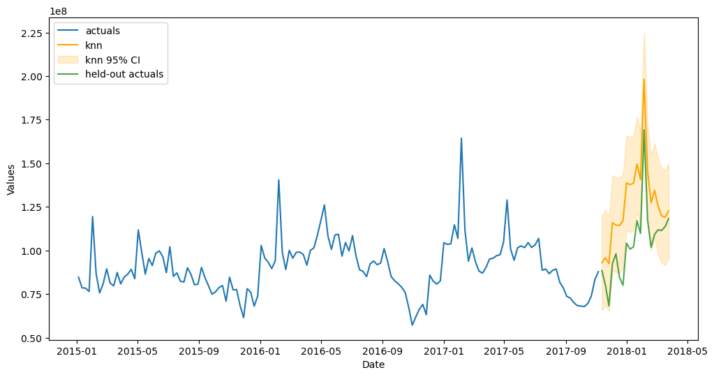
Evaluate Interval
[35]:
fig, ax = plt.subplots(figsize=(12,6))
f.plot(ci=True,models='top_1',order_by='TestSetRMSE',ax=ax)
sns.lineplot(
    y = 'Total Volume',
    x = 'Date',
    data = volume_sep.reset_index(),
    ax = ax,
    label = 'held-out actuals',
    color = 'green',
    alpha = 0.7,
)
plt.show()
[36]:
avc_fcsts1 = f.export("lvl_fcsts",cis=True)
avc_results = score_cis(
    results_template.copy(),
    avc_fcsts1,
    'Avocados',
    volume_sep,
    volume,
    val_len = val_len,
    models = models,
)
avc_results
[36]:
| Avocados | |
|---|---|
| mlr | 8.55 |
| elasticnet | 8.55 |
| ridge | 8.48 |
| knn | 19.70 |
| xgboost | 13.74 |
| lightgbm | 19.81 |
| gbt | 10.65 |
[37]:
results['Avocados'] = avc_results['Avocados']
results
[37]:
| Daily Visitors | Housing Starts | Avocados | |
|---|---|---|---|
| mlr | 5.63 | 5.66 | 8.55 |
| elasticnet | 5.55 | 8.25 | 8.55 |
| ridge | 5.62 | 7.43 | 8.48 |
| knn | 5.64 | 6.55 | 19.70 |
| xgboost | 5.60 | 3.93 | 13.74 |
| lightgbm | 5.20 | 4.29 | 19.81 |
| gbt | 8.32 | 5.88 | 10.65 |
All Aggregated Results
[38]:
_, ax = plt.subplots(figsize=(12,6))
sns.heatmap(
    results,
    annot=True,
    fmt='.2f',
    cmap="Spectral_r",
    ax=ax
)
plt.show()
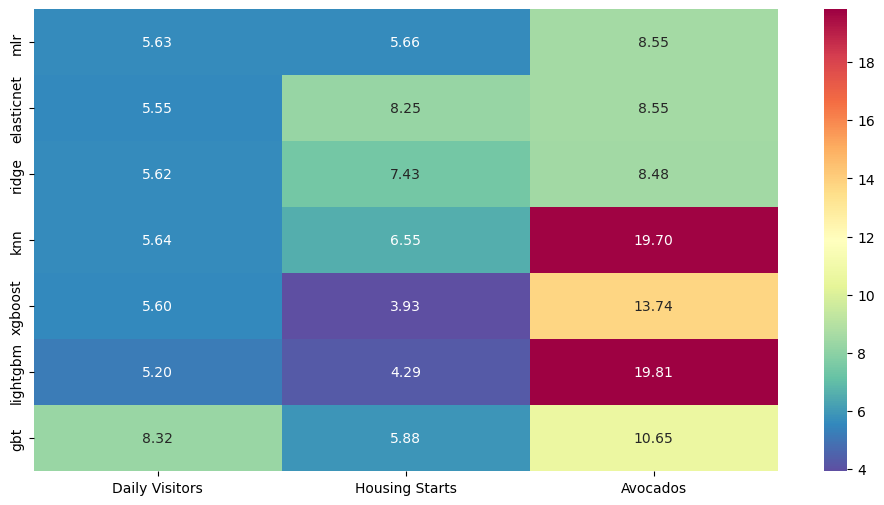
For the most part, the linear models set the best intervals and the boosted tree models were very good or very bad, with GBT more towards the bad side.
Benchmark Against StatsModels ARIMA
Confidence intervals come from StatsModels but the auto-ARIMA process is from PMDARIMA.
[39]:
from scalecast.auxmodels import auto_arima
[40]:
all_series = {
    # series,out-of-sample series,seasonal step
    'visitors':[visits,visits_sep,1],
    'housing starts':[starts,starts_sep,12],
    'avocados':[volume,volume_sep,1]
}
arima_conformal_results = pd.DataFrame()
arima_sm_results = pd.DataFrame()
[41]:
for k, v in all_series.items():
    print(k)
    f = Forecaster(
        y=v[0],
        current_dates=v[0].index,
        future_dates=len(v[1]),
        test_length = len(v[1]),
        cis=True,
    )
    auto_arima(f,m=v[2])
    arima_results = f.export("lvl_fcsts",cis=True)
    # scalecast intervals
    arima_conformal_results.loc[k,'MSIS'] = metrics.msis(
        a = v[1].values,
        uf = arima_results['auto_arima_upperci'].values,
        lf = arima_results['auto_arima_lowerci'].values,
        obs = v[0].values,
        m = v[2],
    )
    # statsmodels intervals
    cis = f.regr.get_forecast(len(v[1])).conf_int()
    arima_sm_results.loc[k,'MSIS'] = metrics.msis(
        a = v[1].values,
        uf = cis.T[1],
        lf = cis.T[0],
        obs = v[0].values,
        m = v[2],
    )
visitors
housing starts
avocados
MSIS Results - ARIMA Scalecast
[42]:
# results from the scalecast intervals
arima_conformal_results
[42]:
| MSIS | |
|---|---|
| visitors | 4.97 |
| housing starts | 24.90 |
| avocados | 23.15 |
[43]:
arima_conformal_results.mean()
[43]:
MSIS   17.67
dtype: float64
MSIS Results - ARIMA StatsModels
[44]:
# results from the statsmodels intervals
arima_sm_results
[44]:
| MSIS | |
|---|---|
| visitors | 5.80 |
| housing starts | 5.62 |
| avocados | 19.94 |
[45]:
arima_sm_results.mean()
[45]:
MSIS   10.46
dtype: float64
[46]:
all_results = results.copy()
all_results.loc['arima (conformal)'] =  arima_conformal_results.T.values[0]
all_results.loc['arima (statsmodels) - benchmark'] = arima_sm_results.T.values[0]
all_results = all_results.T
all_results
[46]:
| mlr | elasticnet | ridge | knn | xgboost | lightgbm | gbt | arima (conformal) | arima (statsmodels) - benchmark | |
|---|---|---|---|---|---|---|---|---|---|
| Daily Visitors | 5.63 | 5.55 | 5.62 | 5.64 | 5.60 | 5.20 | 8.32 | 4.97 | 5.80 |
| Housing Starts | 5.66 | 8.25 | 7.43 | 6.55 | 3.93 | 4.29 | 5.88 | 24.90 | 5.62 |
| Avocados | 8.55 | 8.55 | 8.48 | 19.70 | 13.74 | 19.81 | 10.65 | 23.15 | 19.94 |
[47]:
def highlight_rows(row):
    ret_row = ['']*all_results.shape[1]
    for i, c in enumerate(all_results.iloc[:,:-1]):
        if row[c] < row['arima (statsmodels) - benchmark']:
            ret_row[i] = 'background-color: lightgreen;'
        else:
            ret_row[i] = 'background-color: lightcoral;'
    return ret_row

all_results.style.apply(
    highlight_rows,
    axis=1,
)
[47]:
| mlr | elasticnet | ridge | knn | xgboost | lightgbm | gbt | arima (conformal) | arima (statsmodels) - benchmark | |
|---|---|---|---|---|---|---|---|---|---|
| Daily Visitors | 5.632456 | 5.548336 | 5.622506 | 5.639715 | 5.597762 | 5.196714 | 8.319963 | 4.966161 | 5.796559 |
| Housing Starts | 5.661675 | 8.247183 | 7.432564 | 6.552641 | 3.930183 | 4.289493 | 5.884677 | 24.897373 | 5.624803 |
| Avocados | 8.551783 | 8.551783 | 8.478400 | 19.700378 | 13.743804 | 19.810258 | 10.654140 | 23.151315 | 19.944485 |
The above table shows which scalecast intervals performed better or worse than the ARIMA interval. Green scores are better, red are worse. The scalecast conformal intervals were on the whole better, but not always. When comparing ARIMA to ARIMA, the confidence intervals from statsmodels performed slightly worse on one series, slightly better on another, and significantly better on the remaining one. The rest of the models run through scalecast usually beat the ARIMA intervals on all datasets, except housing starts. XGBoost and Lightgbm were the only models to always beat the intervals from StatsModels. On the whole, the scalecast interval has a nice showing against the more traditional interval from ARIMA in the StatsModels package.
[ ]: