Theta

• Read about the theta model

• See the darts implementation

• See the statsmodels implementation

• Download data from GitHub

• Install darts: pip install darts

• See the blog post

Scalecast ports the model from darts, which is supposed to be more accurate and is also easier to maintain.

import pandas as pd
import numpy as np
import matplotlib.pyplot as plt
import seaborn as sns
from scipy import stats
from darts.utils.utils import SeasonalityMode, TrendMode, ModelMode
from scalecast.Forecaster import Forecaster
from scalecast.util import metrics
from scalecast import GridGenerator

train = pd.read_csv('Hourly-train.csv',index_col=0)
test = pd.read_csv('Hourly-test.csv',index_col=0)
y = train.loc['H7'].to_list()
current_dates = pd.date_range(start='2015-01-07 12:00',freq='H',periods=len(y)).to_list()

y_test = test.loc['H7'].to_list()

f = Forecaster(
    y=y,
    current_dates=current_dates,
    metrics = ['smape','r2'],
    test_length = .25,
    future_dates = len(y_test),
    cis = True,
)

f

Forecaster(
    DateStartActuals=2015-01-18T08:00:00.000000000
    DateEndActuals=2015-02-16T11:00:00.000000000
    Freq=H
    N_actuals=700
    ForecastLength=48
    Xvars=[]
    TestLength=240
    ValidationMetric=smape
    ForecastsEvaluated=[]
    CILevel=0.95
    CurrentEstimator=mlr
    GridsFile=Grids
)

f.plot()
plt.show()

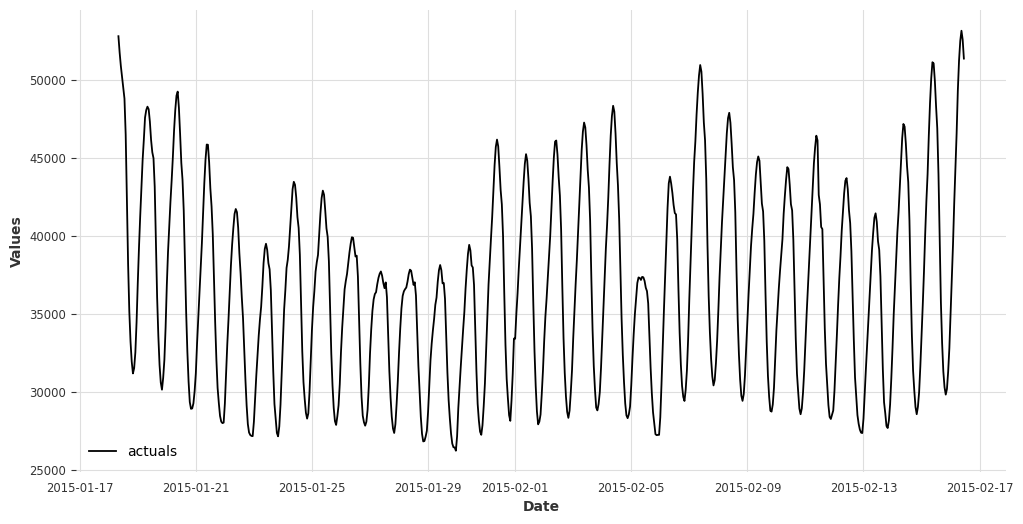
Prepare forecast

• Download theta’s validation grid

GridGenerator.get_grids('theta',out_name='Grids.py')
f.ingest_grid('theta')

Call the forecast

• tune hyperparemters with 3-fold time series cross validation

f.set_estimator('theta')
f.cross_validate(k=3,verbose=True)
f.auto_forecast()

Num hyperparams to try for the theta model: 48.
Fold 0: Train size: 345 (2015-01-18 08:00:00 - 2015-02-01 16:00:00). Test Size: 115 (2015-02-01 17:00:00 - 2015-02-06 11:00:00).
Fold 1: Train size: 230 (2015-01-18 08:00:00 - 2015-01-27 21:00:00). Test Size: 115 (2015-01-27 22:00:00 - 2015-02-01 16:00:00).
Fold 2: Train size: 115 (2015-01-18 08:00:00 - 2015-01-23 02:00:00). Test Size: 115 (2015-01-23 03:00:00 - 2015-01-27 21:00:00).
Chosen paramaters: {'theta': 0.5, 'model_mode': <ModelMode.ADDITIVE: 'additive'>, 'season_mode': <SeasonalityMode.MULTIPLICATIVE: 'multiplicative'>, 'trend_mode': <TrendMode.EXPONENTIAL: 'exponential'>}.

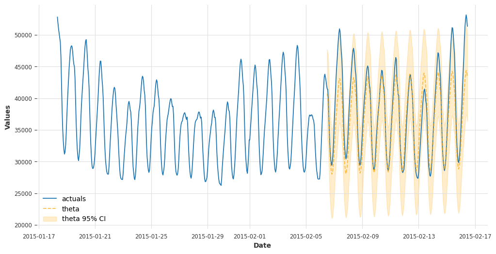
Visualize test results

f.plot_test_set(ci=True)
plt.show()

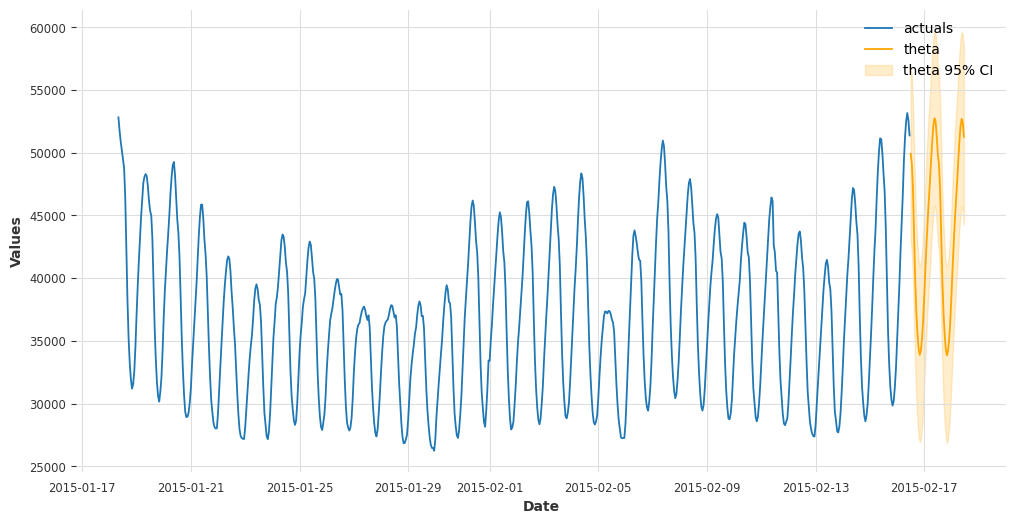
Visualize forecast results

f.plot(ci=True)
plt.show()

See in-sample and out-of-sample accuracy/error metrics

results = f.export('model_summaries')

results[
    [
        'TestSetSMAPE',
        'InSampleSMAPE',
        'TestSetR2',
        'InSampleR2',
        'ValidationMetric',
        'ValidationMetricValue',
        'TestSetLength'
    ]
]

	TestSetSMAPE	InSampleSMAPE	TestSetR2	InSampleR2	ValidationMetric	ValidationMetricValue	TestSetLength
0	0.058274	0.014082	0.786943	0.984652	smape	0.064113	240

The validation metric displayed above is the average SMAPE across the three cross-validation folds.

validation_grid = f.export_validation_grid('theta')
validation_grid.head()

	theta	model_mode	season_mode	trend_mode	Fold0Metric	Fold1Metric	Fold2Metric	AverageMetric	MetricEvaluated
0	0.5	ModelMode.ADDITIVE	SeasonalityMode.MULTIPLICATIVE	TrendMode.EXPONENTIAL	0.056320	0.067335	0.068684	0.064113	smape
1	0.5	ModelMode.ADDITIVE	SeasonalityMode.MULTIPLICATIVE	TrendMode.LINEAR	0.056510	0.072710	0.084188	0.071136	smape
2	0.5	ModelMode.ADDITIVE	SeasonalityMode.ADDITIVE	TrendMode.EXPONENTIAL	0.055679	0.075179	0.073782	0.068213	smape
3	0.5	ModelMode.ADDITIVE	SeasonalityMode.ADDITIVE	TrendMode.LINEAR	0.056044	0.081705	0.089734	0.075827	smape
4	0.5	ModelMode.MULTIPLICATIVE	SeasonalityMode.MULTIPLICATIVE	TrendMode.EXPONENTIAL	0.056569	0.071406	0.080493	0.069489	smape

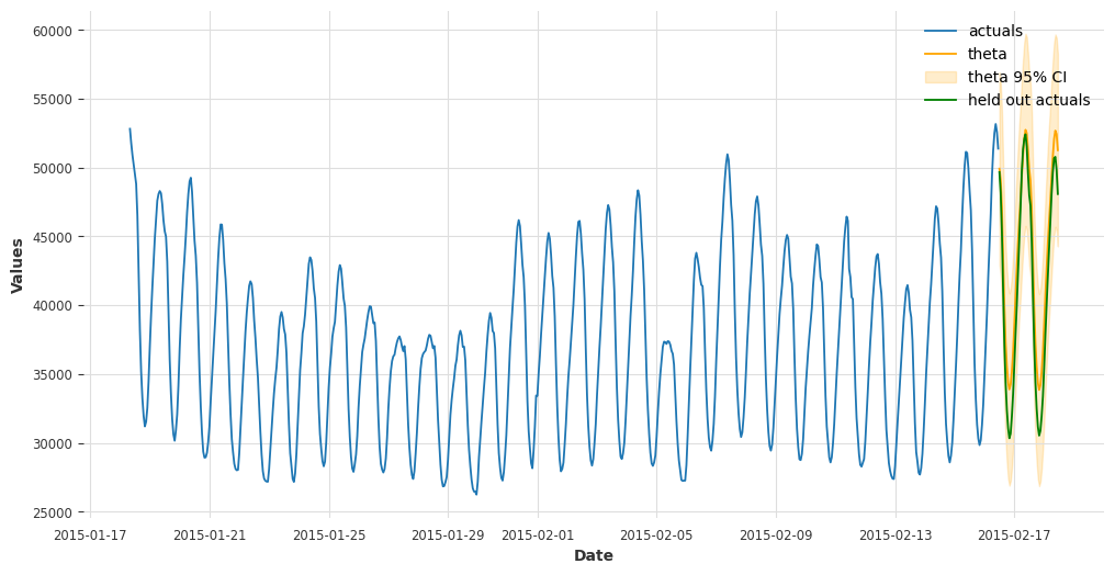
Test the forecast against out-of-sample data

• this is data the Forecaster object has never seen

fcst = f.export('lvl_fcsts')
fcst.head()

	DATE	theta
0	2015-02-16 12:00:00	49921.533332
1	2015-02-16 13:00:00	49135.400143
2	2015-02-16 14:00:00	47126.062514
3	2015-02-16 15:00:00	43417.987575
4	2015-02-16 16:00:00	39867.287257

fig, ax = plt.subplots(figsize=(12,6))
f.plot(ax=ax,ci=True)
sns.lineplot(
    x = f.future_dates,
    y = y_test,
    ax = ax,
    label = 'held out actuals',
    color = 'green',
)
plt.show()

smape = metrics.smape(y_test,fcst['theta'])
smape

0.05764507814606441