RNN and LSTM
This notebook demonstrates the capabilities of the RNN model in scalecast.
Download data: https://www.kaggle.com/robervalt/sunspots
Requirements for this notebook:
pip install tensorflow!pip install tqdm!pip install ipython!pip install ipywidgets!jupyter nbextension enable --py widgetsnbextensionif using Jupyter Lab:
!jupyter labextension install @jupyter-widgets/jupyterlab-manager
[1]:
import pandas as pd
import numpy as np
import pandas_datareader as pdr
import matplotlib
import matplotlib.pyplot as plt
import seaborn as sns
from tqdm.notebook import tqdm
from dateutil.relativedelta import relativedelta
from scalecast.Forecaster import Forecaster
[2]:
df = pd.read_csv('Sunspots.csv',index_col=0,names=['Date','Target'],header=0)
f = Forecaster(
    y=df['Target'],
    current_dates=df['Date'],
    test_length = 240,
    future_dates = 240,
    cis = True,
)
f
[2]:
Forecaster(
    DateStartActuals=1749-01-31T00:00:00.000000000
    DateEndActuals=2021-01-31T00:00:00.000000000
    Freq=M
    N_actuals=3265
    ForecastLength=240
    Xvars=[]
    TestLength=240
    ValidationMetric=rmse
    ForecastsEvaluated=[]
    CILevel=0.95
    CurrentEstimator=mlr
    GridsFile=Grids
)
EDA
[3]:
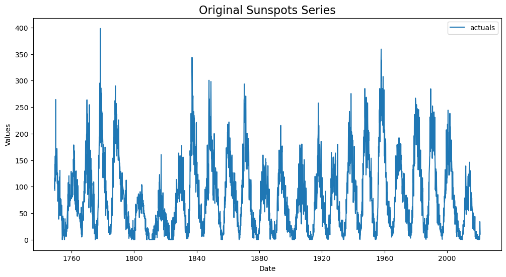
f.plot()
plt.title('Original Sunspots Series',size=16)
[3]:
Text(0.5, 1.0, 'Original Sunspots Series')
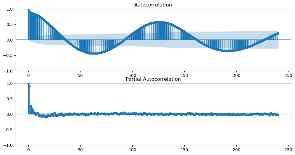
Let’s see the ACF and PACF plots, allowing 240 lags to see this series’ irregular 10-year cycle.
[4]:
figs, axs = plt.subplots(2, 1, figsize = (12,6))
f.plot_acf(ax=axs[0],lags=240)
f.plot_pacf(ax=axs[1],lags=240,method='ywm')
plt.show()
Let’s view the series’ seasonal decomposition.
[5]:
plt.rc("figure",figsize=(10,6))
f.seasonal_decompose().plot()
plt.show()
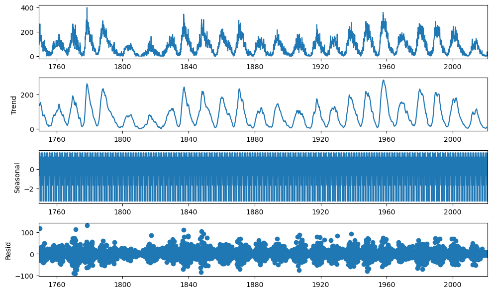
It is very difficult to make out anything useful from this graph.
Forecast RNN Model
See Darts’ GRU on the same series: https://unit8co.github.io/darts/examples/04-RNN-examples.html?highlight=sunspots
SimpleRNN
Unlayered model
1 hidden layer with 20% dropout
25 epochs
20% validcation split
32 batch size
Tanh activation
Adam optimizer
MAE loss function
[6]:
f.auto_Xvar_select(
    try_trend = False,
    irr_cycles = [120,132,144],
    cross_validate = True,
    cvkwargs = {'k':3},
    dynamic_tuning = 240,
)
f.set_estimator('rnn')
f
[6]:
Forecaster(
    DateStartActuals=1749-01-31T00:00:00.000000000
    DateEndActuals=2021-01-31T00:00:00.000000000
    Freq=M
    N_actuals=3265
    ForecastLength=240
    Xvars=['AR1', 'AR2', 'AR3', 'AR4', 'AR5', 'AR6', 'AR7', 'AR8', 'AR9', 'AR10', 'AR11', 'AR12', 'AR13', 'AR14', 'AR15', 'AR16', 'AR17', 'AR18', 'AR19', 'AR20', 'AR21', 'AR22', 'AR23', 'AR24', 'AR25', 'AR26', 'AR27', 'AR28', 'AR29', 'AR30', 'AR31', 'AR32', 'AR33', 'AR34', 'AR35', 'AR36', 'AR37', 'AR38', 'AR39', 'AR40', 'AR41', 'AR42', 'AR43', 'AR44', 'AR45', 'AR46', 'AR47', 'AR48', 'AR49', 'AR50', 'AR51', 'AR52', 'AR53', 'AR54', 'AR55', 'AR56', 'AR57', 'AR58', 'AR59', 'AR60', 'AR61', 'AR62', 'AR63', 'AR64', 'AR65', 'AR66', 'AR67', 'AR68', 'AR69', 'AR70', 'AR71', 'AR72', 'AR73', 'AR74', 'AR75', 'AR76', 'AR77', 'AR78', 'AR79', 'AR80', 'AR81', 'AR82', 'AR83', 'AR84', 'AR85', 'AR86', 'AR87', 'AR88', 'AR89', 'AR90', 'AR91', 'AR92', 'AR93', 'AR94', 'AR95', 'AR96', 'AR97', 'AR98', 'AR99', 'AR100', 'AR101', 'AR102', 'AR103', 'AR104', 'AR105', 'AR106', 'AR107', 'AR108', 'AR109', 'AR110', 'AR111', 'AR112', 'AR113', 'AR114', 'AR115', 'AR116', 'AR117', 'AR118', 'AR119', 'AR120', 'AR121', 'AR122', 'AR123', 'AR124', 'AR125', 'AR126', 'AR127', 'AR128', 'AR129', 'AR130', 'AR131', 'AR132', 'AR133', 'AR134', 'AR135', 'AR136', 'AR137', 'AR138', 'AR139', 'AR140', 'AR141', 'AR142', 'AR143', 'AR144', 'AR145', 'AR146', 'AR147', 'AR148', 'AR149', 'AR150', 'AR151', 'AR152', 'AR153', 'AR154', 'AR155', 'AR156', 'AR157', 'AR158', 'AR159', 'AR160', 'AR161', 'AR162', 'AR163', 'AR164', 'AR165', 'AR166', 'AR167', 'AR168', 'AR169', 'AR170', 'AR171', 'AR172', 'AR173', 'AR174', 'AR175', 'AR176', 'AR177', 'AR178', 'AR179', 'AR180', 'AR181', 'AR182', 'AR183', 'AR184', 'AR185', 'AR186', 'AR187', 'AR188', 'AR189', 'AR190', 'AR191', 'AR192', 'AR193', 'AR194', 'AR195', 'AR196', 'AR197', 'AR198', 'AR199', 'AR200', 'AR201', 'AR202', 'AR203', 'AR204', 'AR205', 'AR206', 'AR207', 'AR208', 'AR209', 'AR210', 'AR211', 'AR212', 'AR213', 'AR214', 'AR215', 'AR216', 'AR217', 'AR218', 'AR219', 'AR220', 'AR221', 'AR222', 'AR223', 'AR224', 'AR225', 'AR226', 'AR227', 'AR228', 'AR229', 'AR230', 'AR231', 'AR232', 'AR233', 'AR234']
    TestLength=240
    ValidationMetric=rmse
    ForecastsEvaluated=[]
    CILevel=0.95
    CurrentEstimator=rnn
    GridsFile=Grids
)
[7]:
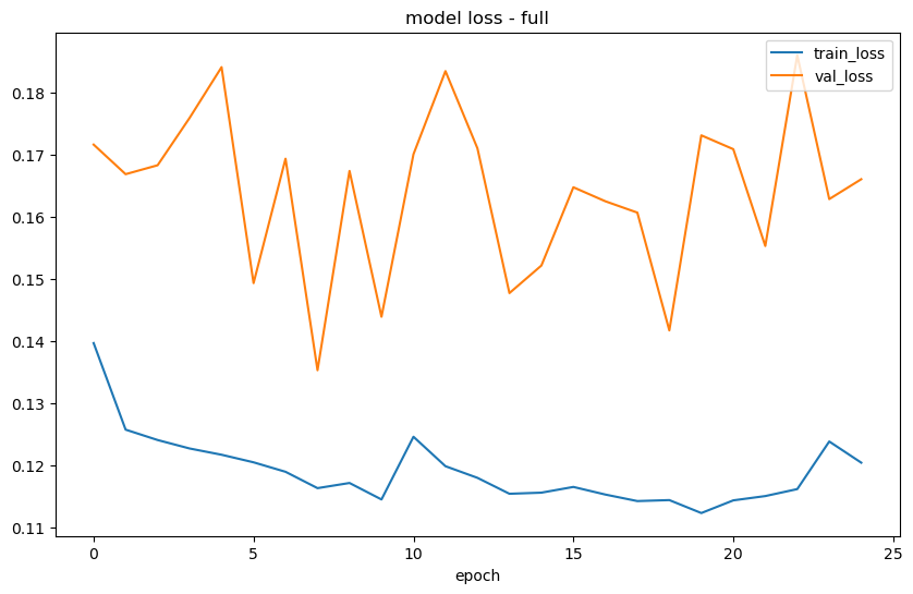
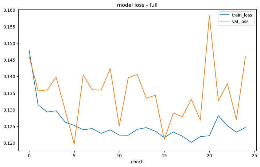
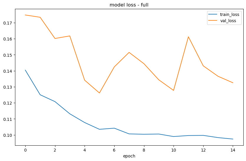
f.manual_forecast(
    layers_struct=[('SimpleRNN',{'units':100,'dropout':0.2})],
    epochs=25,
    validation_split=0.2,
    plot_loss=True,
    call_me="rnn_1layer",
    verbose=0, # so it doesn't print each epoch and saves space in the notebook
)
2023-04-11 16:31:38.533751: I tensorflow/core/platform/cpu_feature_guard.cc:193] This TensorFlow binary is optimized with oneAPI Deep Neural Network Library (oneDNN) to use the following CPU instructions in performance-critical operations:  SSE4.1 SSE4.2
To enable them in other operations, rebuild TensorFlow with the appropriate compiler flags.
2023-04-11 16:31:40.033534: I tensorflow/core/platform/cpu_feature_guard.cc:193] This TensorFlow binary is optimized with oneAPI Deep Neural Network Library (oneDNN) to use the following CPU instructions in performance-critical operations:  SSE4.1 SSE4.2
To enable them in other operations, rebuild TensorFlow with the appropriate compiler flags.
1/1 [==============================] - 0s 108ms/step
1/1 [==============================] - 0s 91ms/step
88/88 [==============================] - 1s 10ms/step
Layered Model
2 SimpleRNN layers, 100 units each
2 Dense layers, 10 units each
No dropout
Everything else the same
[8]:
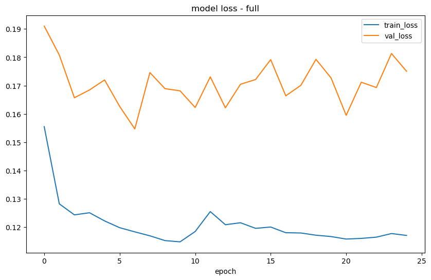
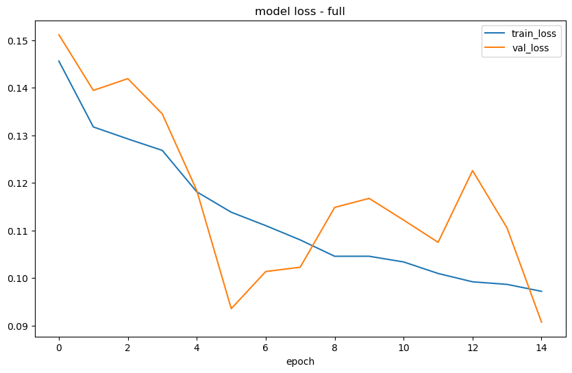
f.manual_forecast(
    layers_struct=[
        ('SimpleRNN',{'units':100,'dropout':0})
    ] * 2 + [
        ('Dense',{'units':10})
    ]*2,
    epochs=25,
    random_seed=42,
    plot_loss=True,
    validation_split=0.2,
    call_me='rnn_layered',
    verbose=0
)
1/1 [==============================] - 0s 150ms/step
1/1 [==============================] - 0s 154ms/step
88/88 [==============================] - 2s 19ms/step
[9]:
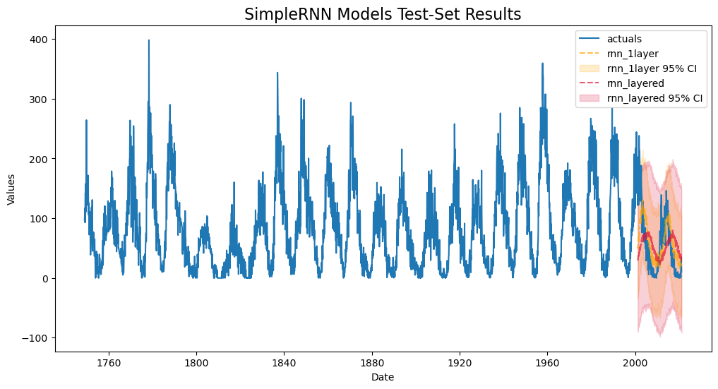
f.plot_test_set(
    ci=True,
    models=['rnn_1layer','rnn_layered'],
    order_by='TestSetRMSE',
)
plt.title('SimpleRNN Models Test-Set Results',size=16)
plt.show()
LSTM
Unlayered Model
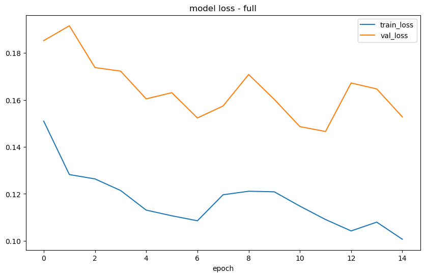
One LSTM layer with 20% dropout
15 epochs
Everything else the same
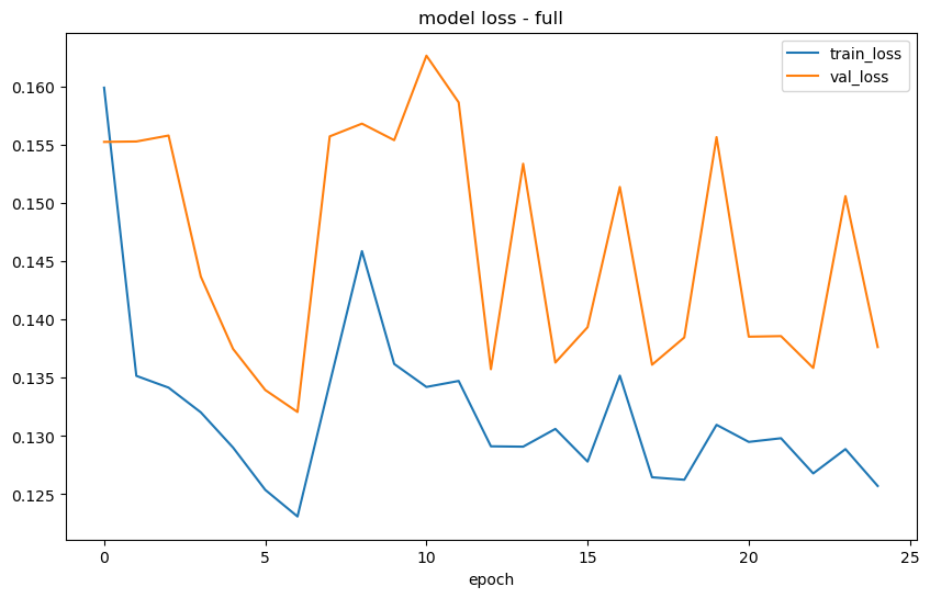
[10]:
f.manual_forecast(
    layers_struct=[('LSTM',{'units':100,'dropout':0.2})],
    epochs=15,
    validation_split=0.2,
    plot_loss=True,
    call_me="lstm_1layer",
    verbose=0, # so it doesn't print each epoch and saves space in the notebook
)
1/1 [==============================] - 0s 216ms/step
1/1 [==============================] - 0s 219ms/step
88/88 [==============================] - 3s 29ms/step
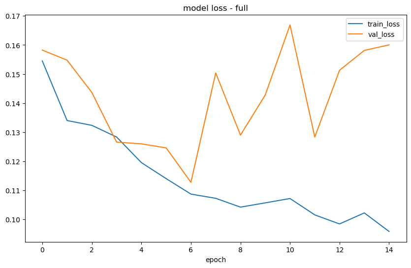
Layered Model
2 lstm layers and 2 dense layers
No dropout
[11]:
f.manual_forecast(
    layers_struct=[
        ('LSTM',{'units':100,'dropout':0})
    ] * 2 + [
        ('Dense',{'units':10})
    ] * 2,
    epochs=15,
    random_seed=42,
    plot_loss=True,
    validation_split=0.2,
    call_me='lstm_layered',
    verbose=0
)
1/1 [==============================] - 0s 408ms/step
1/1 [==============================] - 0s 411ms/step
88/88 [==============================] - 5s 59ms/step
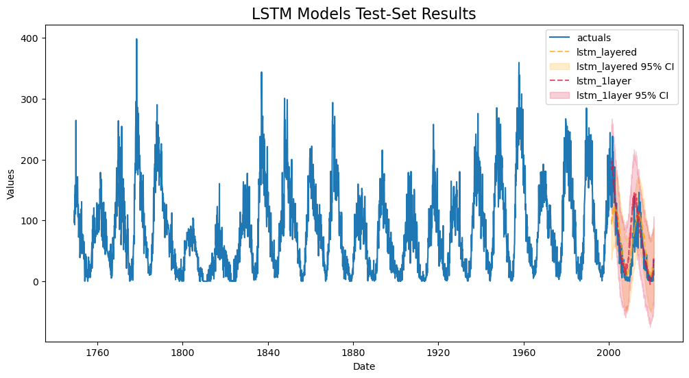
[12]:
f.plot_test_set(models=['lstm_1layer','lstm_layered'],ci=True,order_by='TestSetRMSE')
plt.title('LSTM Models Test-Set Results',size=16)
plt.show()
Prepare NNAR Model
Let’s try building a model you can read about here: https://otexts.com/fpp2/nnetar.html
This is a time-series based dense neural network model, where the final predictions are the average of several models with randomly selected starting weights
It is not a recurrent neural network and does not use the rnn estimator, but I thought it’d be fun to demonstrate here.
It takes three input parameters:
p (number of lags)
P (number of seasonal lags)
m (seasonal period)
It also accepts exogenous variables. We add a time trend, monthly seasonality in wave functions, and a 120-period cycle
Another parameter to consider is k: the size of the hidden layer. By default, this is the total number of inputs divided by 2, rounded up. We will keep the default
The default number of models to average is 20 and we will keep that default as well
See the model’s documentation in R: https://www.rdocumentation.org/packages/forecast/versions/8.16/topics/nnetar
[13]:
p = 10 # non-seasonal lags
P = 6  # seasonal lags
m = 12 # seasonal period

f.drop_all_Xvars()
f.add_ar_terms(p)
f.add_AR_terms((P,m))

# in addition to the process described in the linked book, we can add monthly seasonality in a fourier transformation
f.add_seasonal_regressors('month',raw=False,sincos=True)
# lastly, we add an irregular 10-year cycle that is idionsycratic to this dataset
f.add_cycle(120)
[14]:
f
[14]:
Forecaster(
    DateStartActuals=1749-01-31T00:00:00.000000000
    DateEndActuals=2021-01-31T00:00:00.000000000
    Freq=M
    N_actuals=3265
    ForecastLength=240
    Xvars=['AR1', 'AR2', 'AR3', 'AR4', 'AR5', 'AR6', 'AR7', 'AR8', 'AR9', 'AR10', 'AR12', 'AR24', 'AR36', 'AR48', 'AR60', 'AR72', 'monthsin', 'monthcos', 'cycle120sin', 'cycle120cos']
    TestLength=240
    ValidationMetric=rmse
    ForecastsEvaluated=['rnn_1layer', 'rnn_layered', 'lstm_1layer', 'lstm_layered']
    CILevel=0.95
    CurrentEstimator=rnn
    GridsFile=Grids
)
Forecast NNAR Model
[15]:
# the default parameter used in the book is the total number of inputs divided by 2, rounded up
k = int(np.ceil(len(f.get_regressor_names())/2))
repeats = 20 # default repeats number used in book
f.set_estimator('mlp')
for r in tqdm(range(repeats)): # repeats
    f.manual_forecast(
        hidden_layer_sizes=(k,),
        activation='relu',
        random_state=r,
        normalizer='scale',
        call_me=f'mlp_{r}',
    )
f.save_feature_importance()
# now we take the averages of all models to create the final NNAR
f.set_estimator('combo')
f.manual_forecast(how='simple',models=[f'mlp_{r}' for r in range(20)],call_me='nnar')
[16]:
f.plot_test_set(ci=True,models='nnar')
plt.title('NNAR Test-Set Performance',size=16)
plt.show()
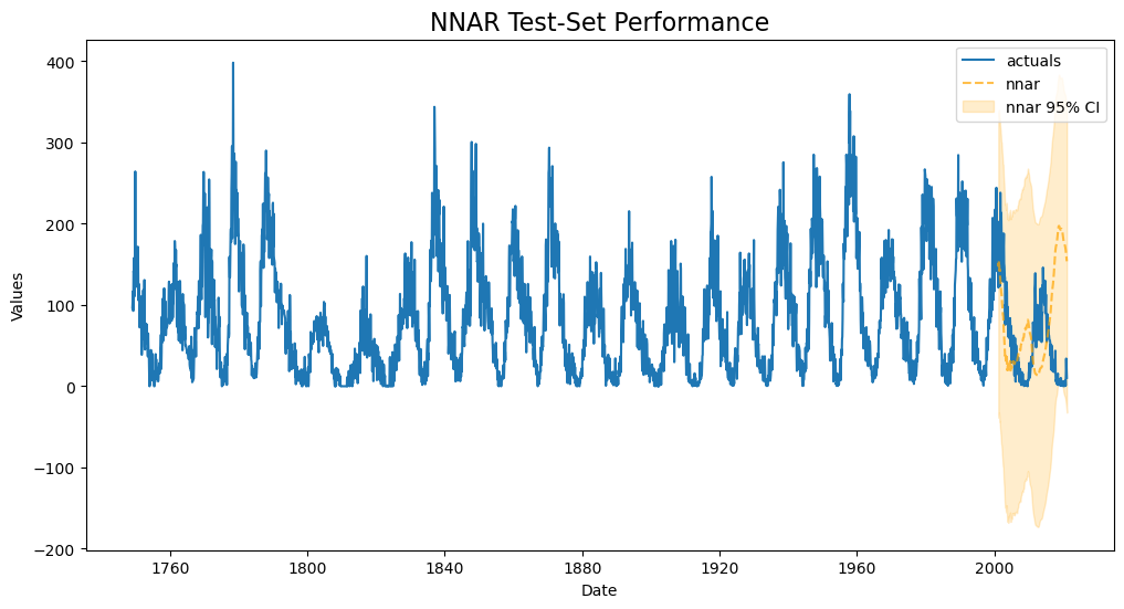
This doesn’t look as good as any of our evaluated RNN models.
One thing we notice with all these test-set graphs is that the precise deviations from the trend are hard to see because the series is so large. Let’s call the function again with all evaluated models ordered by test RMSE and zoomed in to the test-set section of the series only by setting include_train=False.
[17]:
f.plot_test_set(
    models=['rnn_1layer','rnn_layered','lstm_1layer','lstm_layered','nnar'],
    order_by='TestSetRMSE',
    include_train=False,
)
plt.title('All Models Test Performance - test set obs only',size=16)
plt.show()
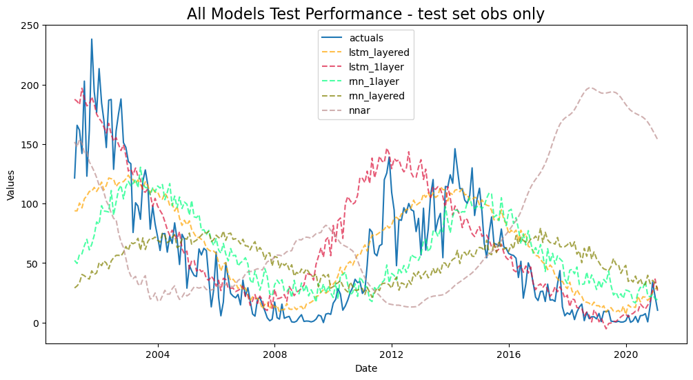
With this view, it is not clear that any model did as well as we might have thought from the other graphs.
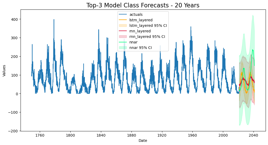
Compare All Models
Forecast Plot
best rnn model
best lstm model
nnar model
[18]:
f.plot(models=['rnn_layered','lstm_layered','nnar'],order_by='TestSetRMSE',ci=True)
plt.title('Top-3 Model Class Forecasts - 20 Years',size=16)
plt.show()
Export Model Summaries for all applied models
[19]:
pd.set_option('display.float_format',  '{:.4f}'.format)
f.export(
    'model_summaries',
    models=['rnn_1layer','rnn_layered','lstm_1layer','lstm_layered','nnar'],
    determine_best_by = 'TestSetRMSE',
)[
    [
        'ModelNickname',
        'TestSetRMSE',
        'TestSetR2',
        'InSampleRMSE',
        'InSampleR2',
        'best_model'
    ]
]
[19]:
| ModelNickname | TestSetRMSE | TestSetR2 | InSampleRMSE | InSampleR2 | best_model | |
|---|---|---|---|---|---|---|
| 0 | lstm_layered | 28.5508 | 0.7083 | 56.6811 | 0.3310 | True |
| 1 | lstm_1layer | 31.8674 | 0.6366 | 43.3984 | 0.6078 | False |
| 2 | rnn_1layer | 41.2311 | 0.3918 | 68.7316 | 0.0163 | False |
| 3 | rnn_layered | 55.6165 | -0.1067 | 60.6494 | 0.2341 | False |
| 4 | nnar | 92.0142 | -2.0293 | 28.4102 | 0.8266 | False |
Backtest Best Model
The LSTM with four layers appears to be our most accurate model out of the 5 we ran and showed. The NNAR model, in spite of being fun to set up, was the worst. With more time spent, even better results could be extracted. Although that model appears accurate on the test set we gave to it, an interesting question is how good it would have been if we had used it in production for the last 5 years. That’s what backtesting allows us to evaluate. Backtesting can take a long time for more complex models.
[32]:
from scalecast.Pipeline import Pipeline
from scalecast.util import backtest_metrics

def forecaster(f):
    f.auto_Xvar_select(
        try_trend = False,
        irr_cycles = [120,132,144],
        cross_validate = True,
        cvkwargs = {'k':3},
        dynamic_tuning = 240,
        max_ar = 240,
    )
    f.set_estimator('rnn')
    f.manual_forecast(
        layers_struct=[
            ('LSTM',{'units':100,'dropout':0})
        ] * 2 + [
            ('Dense',{'units':10})
        ] * 2,
        epochs=15,
        random_seed=42,
        validation_split=0.2,
        call_me='lstm_layered',
        verbose=0
    )

pipeline = Pipeline(steps = [('Forecast',forecaster)])
[33]:
# default args below
backtest_results = pipeline.backtest(
    f,
    n_iter=5,
    fcst_length = 240,
    test_length = 0,
    jump_back = 12, # place a year between consecutive training sets
    cis = False,
)
bm = backtest_metrics(backtest_results,mets=['r2','rmse'])
bm
1/1 [==============================] - 0s 439ms/step
80/80 [==============================] - 5s 63ms/step
1/1 [==============================] - 0s 418ms/step
80/80 [==============================] - 5s 67ms/step
1/1 [==============================] - 0s 414ms/step
79/79 [==============================] - 5s 67ms/step
1/1 [==============================] - 0s 435ms/step
79/79 [==============================] - 6s 70ms/step
1/1 [==============================] - 0s 390ms/step
80/80 [==============================] - 5s 58ms/step
[33]:
| Iter0 | Iter1 | Iter2 | Iter3 | Iter4 | Average | ||
|---|---|---|---|---|---|---|---|
| Model | Metric | ||||||
| lstm_layered | r2 | 0.7385 | 0.3077 | 0.3695 | 0.3589 | 0.2503 | 0.4050 |
| rmse | 27.0322 | 48.1908 | 46.7773 | 45.9266 | 49.2748 | 43.4403 |
[34]:
rmse = bm.loc[('lstm_layered','rmse'),'Average']
r2 = bm.loc[('lstm_layered','r2'),'Average']

print(
    'This shows that if we had used this model on actual data in the previous 5 years,'
    f' it would have obtained an average RMSE of {rmse:.1f} and R2 of {r2:.1%}.'
)
This shows that if we had used this model on actual data in the previous 5 years, it would have obtained an average RMSE of 43.4 and R2 of 40.5%.
[ ]: